effective n,k retrevial

Metamaterial S parameter extraction

Metamaterial

This page describes how to calculate the meta-material S parameters of a metamaterial device.

Understanding S parameters

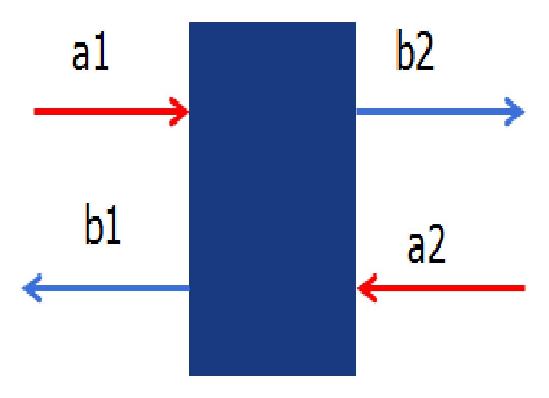
S parameters describe behaviors of a 2 by 2 network or transmission lines (see the figure below):

S parameters for a 2 port network

for two given input signals a1a1 and a2a2, the outputs b1b1 and b2b2 can be calculated as

(b1b2)=(S11S12S21S22)(a1a2)(b1b2)=(S11S12S21S22)(a1a2)

Measuring S parameters from your FDTD simulation

S parameters are complex amplitude reflection and transmission coefficients (in contrast to the power reflection and transmission coefficients). For example, S11S11 is the reflection coefficient and S21S21 is the transmission coefficient for a1a1 incidence; and S22S22 is the reflection coefficient and S12S12 is the transmission coefficient for a2a2 incidence.

Phase compensation for source and monitors

Recognizing that the a,b coefficients are directly proportional to the electric fields, the S parameters can be calculated from the definition above, eg, S11=b1/a1=Er/EiS11=b1/a1=Er/Ei and S21=b2/a1=Et/EiS21=b2/a1=Et/Ei where Ei,Er,EtEi,Er,Et are the incident, reflected and transmitted electric fields. This technique makes it very simple to obtain S-parameters for a given device, but it does make a number of assumptions. It’s important to ensure that all of the assumptions are valid for your simulation.

  • To measure the S parameters in the near field (as done in the S parameter analysis object), the transmitted and reflected fields must be propagating like a simple plane wave at the point of measurement.  The measurements will not be correct if evanescent fields are present. To avoid the evanescent fields, make sure the monitor is sufficiently far from the structure.
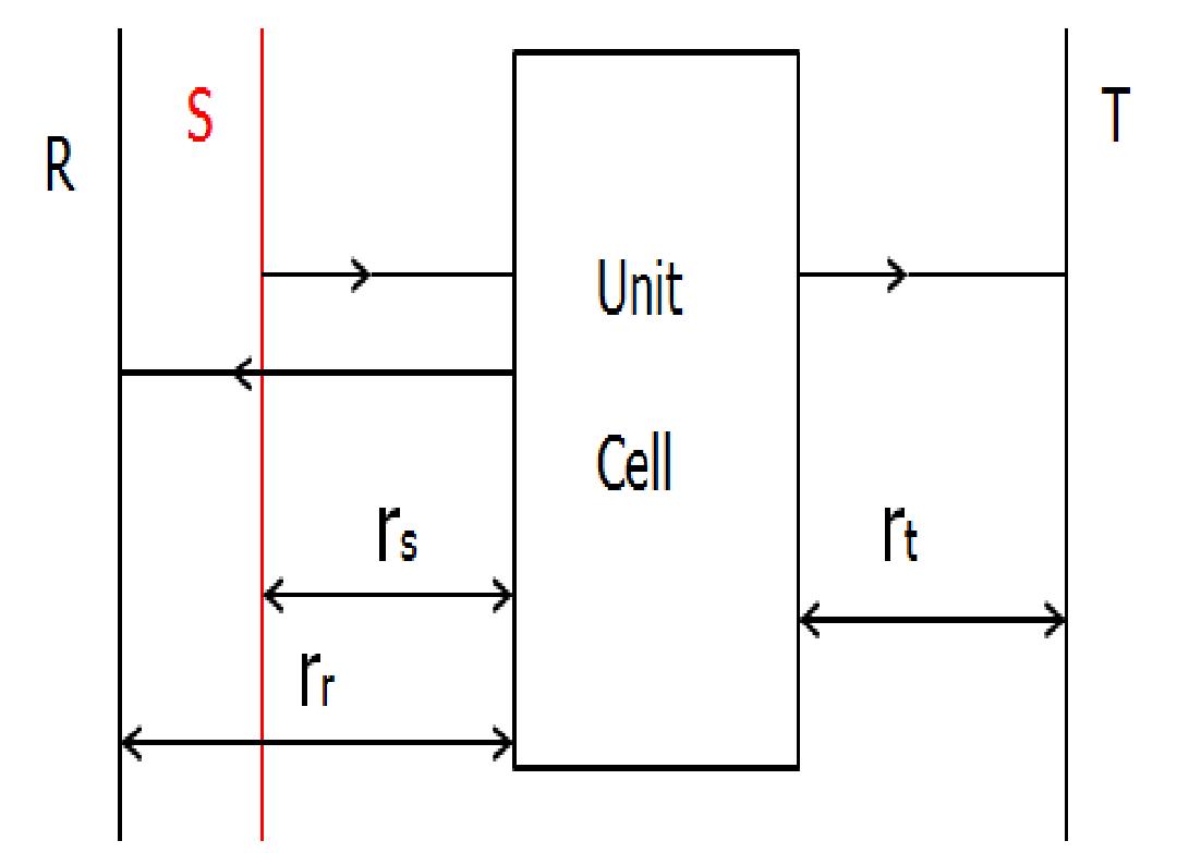
  • In your simulation, the sources and monitors are always some distance from the surface of the metamaterial (for example, the monitors must be far enough from the structure to avoid evanescent fields). The fields will accumulate additional phase as they propagate from the source to the metamaterial, and from the metamaterial to the monitors.  The S parameters are intended to characterize only the metamaterial, without this additional propagation phase, thus we must compensate this additional phase. Suppose the wavenumber in the incidence space is ki, and the wavenumber in transmission space is kt, the extra phase in Monitor T from source S is  kirs+ktrt where rs and rare distances (so they are positive). For reflection Monitor R, the extra phase from source S is  kirs+kirr .

Based on the above discussion, a ready-to-use grating S Parameters analysis group is available in the Object Library. In most cases you only need to set the slab thickness, the locations of the slab center and source position along x axis, and the background refractive index in Analysis–Variables. The phase compensation is done in the Script. Note that because the reflected and transmitted waves must be propagating like plane waves, we use a point-type frequency-domain monitor, to record the electric field component. The analysis group also contains two 2D surface-monitors, which are used to measure the power transmission and to check that the fields are in fact propagating like a single plane wave.

This analysis group calculates the S parameters (amplitude and phase) of a metamaterial, based on grating projections of the near-field data collected by DFT monitors for transmission and reflection. The analysis group isolates a particular output grating order, which can be selected by the user (see the analysis properties description below). The S parameters are defined so that for a planar structure they match with the Fresnel coefficients, defined according to the convention in Reference [1] (see diagram below). This convention is consistent with the behaviour of the stackrt script command. Therefore, if the media above and below the metamaterial have different refractive indices, |S12|2|S12|2  and |S21|2|S21|2 can be larger than 1. The analysis group can handle oblique incidence and s and p-polarized light for input and output.

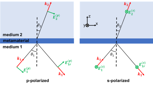
Fig.1 Convention for s- and p-polarized light used in S parameter calculation.

This analysis group has several setup properties, which are described in detail in the setup script inside the object. Here it is worth mentioning:

  • “start wavelength” and “stop wavelength”, which specify the wavelength range of the source. If the start and stop wavelength are not the same, the number of frequency points used can be set in the global monitor properties.
  • “source_type”, which is used to select between two types of sources: 1 for Bloch/periodic and 2 for BFAST. Only use “source_type” = 2 for broadband simulations at oblique incidence (see Source – BFAST). In the present example, we will consider normal incidence only and so we set “source_type” = 1.

In addition, it is important to set the following analysis properties (for more information refer to the information in the analysis script of “s_params_adv”):

  • “metamaterial center” and “metamaterial span” specify the region that you consider to be the metamaterial in global coordinates. This information is used to subtract an additional phase to the S parameters due to the location of the source and the hemisphere where the far-field is calculated. This is similar to the phase correction procedure described here.
  • “target_grating_order_out” specifies the particular output grating order that will be considered to calculate the S parameters.
  • “suppress_warnings” disables (suppress_warnings = 1) or enables (supress_warnings = 0) pop-up windows with warning messages (see description below). If warnings are generated, the “warnings” result will be 1.

Warnings will be generated if:

  • The polarization of the source is not either S or P.
  • The desired order was not found for some of the frequency points. This will happen when the target grating order is not supported.

The analysis group generates two S-parameter results: “S” and “S_polarization”. The first one is the S parameter for dominant input polarization and the same output polarization (e.g. if the source is s-polarized, it will calculate the result only for the s-polarized transmitted and reflected light). The second one is the S parameter for dominant input polarization and both output polarizations, which is only useful when we expect the polarization to be rotated by the metamaterial. In the simple case considered here, there is no polarization rotation and so we can simply use the “S” result and its attributes: “S11_Gn” and “S21_Gn” (source in medium 1) and “S22_Gn” and “S12_Gn” (source in medium 2).

Related publications

  1. D. R. Smith et al., “Electromagnetic parameter retrieval from inhomogeneous metamaterials”, Phys Rev E 71, 036617 (2005)
  2. Szabó, Z., G.-H. Park, R. Hedge, and E.-P. Li, “A unique extraction of metamaterial parameters based on Kramers-Kronig relationship,” IEEE MTT, vol. 58, no. 10, 2010, pp. 2646-2653
  3. P. Yeh, “Optical Waves in Layered Media”, Wiley-InterScience, chap. 3, 2005.

A Unique Extraction of Metamaterial Parameters Based on Kramers–Kronig Relationship

Comments on “A Unique Extraction of Metamaterial
Parameters Based on Kramers–Kronig Relationship”

RefFIT program: fit optical spectra,

https://reffit.ch/

RefFIT is a data analysis program written by dr. Alexey Kuzmenko using the input and feedback from many colleagues over many years. It is designed to fit optical spectra, such as reflectivity, transmission, ellipsometry and Kerr and Faraday rotation using the Drude-Lorentz, Fano, Tauc-Lorentz and many other dielectric-function models. Currently the library includes more than 50 models. In addition to the rich model library, RefFIT allows you to apply a model-independent Kramers-Kronig analysis to virtually any type of optical spectra, using an original Kramers-Kronig constrained variational technique.

RefFIT has a powerful and fast fitting engine based on a modified Levenberg-Marquardt algorithm, a broad collection of proven physical models and a unique user-friendly interface. It allows you fitting manually or automatically several datasets of different type and using different models simultaneously while seeing on your screen precisely what you are doing.

Our users include physicists, material scientists, chemists, optics engineers, biologists and even computer-game designers. Also teachers use RefFIT in their courses: students can not only study the optical properties of materials, they themselves can play, model and fit as well.

Software KK

The software from the division is free to use. The coder should however be acknowledged if the use results in published scientific work.  

https://materialvetenskap.uu.se/research/solid-state-physics+/Software/

KKKTON – A program for Kramers-Kronig (KK) analysis of optical data.

Multifresnel_general – A program for thin film optics calculations. Contains the main program library that is needed for all multifresnel programs listed.

Mulifresnel_sol_vis – Incluces solar and luminous values into the optical calculations.

RT_Invert – A program for calculations of optical constants from experimental data. This program uses the mulitfresnel library.

RT_Invert-variant – A program for calculations of optical constants from the raw data files from the spectrophotometer. This program uses the mulitfresnel library.raw data using the mulitfresnel library.

nk-felyta – Calculates all possible optical constants values from experimental data. Can be used as an aid to determine possible solutions. This program uses the mulitfresnel library.

KKKTON – A PROGRAM FOR KRAMERS-KRONIG (KK) ANALYSIS OF OPTICAL DATA.

The KK analysis is carried out using the extinction coefficient (k) as input and the refractive index (n) is calculated. Low energy Drude and high-energy Lorentz extrapolations are used and parameters for these need also to be inputs. The Matlab program contains a routine for calculating reflectance (R) and transmittance (T) for a film on a substrate and comparing with experimental R and T that need to be entered into the program. kdata.txt is an example of an input file of k-data. See attached files for detailed instructions and program files.

Coder: Annette Hultåker

“MULTIFRESNEL_GENERAL” PROGRAM: THIN FILM OPTICS CALCULATIONS.

This program calculates reflectance, back reflectance and transmittance for a stack of thin films on a substrate. The multilayer stack can have an arbitrary number of layers. A thin film optics formalism using layer and interface matrices is used (P. Pfrommer et al. Sol. Energy, vol 54, No 5, pp. 287-299). The layers can be either coherent or non-coherent, while the substrate is always non-coherent.

Inputs are wavelength (nm), refractive index and extinction coefficient (n and k; from files) for each layer and the substrate, as well as thicknesses (nm), angle of incidence and whether the layers are coherent or not. Wavelength interval and substrate thickness can be adjusted directly in the code.

Output data are plotted in a figure and saved in file ”calcspectra.txt”

Warning: Numerical errors can occur for thick substrates with significant absorption.

The main program calls a number of functions, where different parts of the calculations are carried out. These are:

RT_calc.m  –  Calculates reflectance and transmittance for s-, p- and unpolarized light from the transfer matrix.
transfer_matrix.m  –  Calculates the transfer matrix of the multilayer.
rt2RT.m  –  Calculates reflectance and transmittance from reflection and transmission coefficients.
coherent_l.m  –  Calculates the layer matrix of a coherent layer.
coherent_i.m  –  Calculates the corresponding interface matrix.
non-coherent_L.m  –  Calculates the layer matrix of a non-coherent layer.
non-coherent_I.m  –  Calculates the corresponding interface matrix.
Fresnel_calc.m  –  Calculates Fresnel reflection and transmission coefficients at an interface for s- and p-polarized light.
theta_calc.m  –  Calculates the local angle of incidence at each layer.
mult_3D.m  –  Function for multiplying 3D matrices required for optical calculations.

Note: These functions are also used in all our thin film optics programs on this webpage. By modifying the main program one can use the calculations of the functions for different purposes, for example solving the inverse problem of obtaining optical constants of one layer from experimental data.

MULTIFRESNEL_SOLAR_VIS PROGRAM

This version of the multifresnel program does the same basic calculations as the ”general” version, using the same functions that were supplied with ”multifresnel_general”. However the main program has an additional code that computes solar and luminmous transmittance and reflectance by averaging over the AM1.5 solar spectrum and the luminous eye sensitivity spectrum.

Inputs are wavelength (nm), n and k for each layer, as well as thicknesses (nm) and angle of incidence. The substrate optical constants are also needed. The program needs access, in the same folder, to solar AM1.5 (iso9845tot.txt) and eye sensitivity (eye1.txt) spectra.

Coder: Arne Roos, Anna Werner

RT_INVERT – PROGRAM FOR CALCULATIONS OF OPTICAL CONSTANTS.

These programs fit calculations of reflectance and transmittance for an arbitrary stack of thin films, wherein one layer is unknown, to experimental data. This is done in order to determine the optical constants (refractive index (n) and extinction coefficient (k)) of the unknown layer. Before proceeding to the programs a cautionary note is in order. The inverse problem of thin film optics has multiple solutions and one must be careful to check that the program fits to the physical solution, for example by using independent knowledge of the material under study. Furthermore it is common that the results given by the program cross over from one solution to another one at certain points. This behaviour is especially comon at interference fringes. Hence it may be necessary to perform calculations in different wavelength ranges, in order to obtain the physical solution everywhere. These complications makes determination of optical constants by direct inversion somewhat cumbersome.

The programs listed below all use the MATLAB functions listed in the description of the Multifresnel programs. These must be accessible in the same folder as the main programs listed below.

RT_invert_optconst program

This program calculates optical constants of a coherent or non-coherent layer from an input file containing wavelength, transmittance and reflectance data. The unknown film is situated upon a number of underlayers, which can be either coherent or non-coherent and whose optical constants must be known. The layers are numbered from the top and the substrate is the last underlayer. If number of underlayers is put to zero the remaining layer must be coherent.

Input files are interpolated to the same wavelengths (input data must be given in a wider wavelength region than the interpolation range!). The program uses non-linear least squares fitting starting at the shortest wavelength.

The main program calls the function find_nk as well as RT_calc. The latter one uses the other functions in the multifresnel library.

Input: File with experimental wavelength, transmittance and reflectance. Incidence angle, film thickness and coherence of the unknown layer. Number of underlayers. Optical constants, thickness and coherence of each underlayer.

Output: Figures of n and k; experimental and fitted R and T; deviations between experiment and calculations. Wavelength and calculated n.k are saved in a file.

Coder: Jonas Backholm, Arne Roos (edited by Gunnar Niklasson)

RT_INVERT VARIANT – PROGRAM FOR CALCULATING OPTICAL CONSTANTS

This program is identical to the one above with the following exception: It is intended to be used directly with datafiles from the spectrophotometer. Spectrophotometer measurements start at long wavelengths and proceed to shorter ones. This is often an advantage for the inverse problem, since it is often easier to get good convergence of the calculation at long wavelengths and the problem of multiple solutions is at least less severe. Hence this program uses non-linear least squares fitting starting at the longest wavelength.

The main program calls the function find_nk as well as RT_calc. The latter one uses the other functions in the multifresnel library.

Input: File with experimental wavelength, transmittance and reflectance. Incidence angle, film thickness and coherence of the unknown layer. Number of underlayers. Optical constants, thickness and coherence of each underlayer.

Output: Figures of n and k; experimental and fitted R and T; deviation between experiment and calculations. Wavelength and calculated n.k are saved in a file.

Coder: Jonas Backholm, Arne Roos

NK_FELYTA – CALCULATES ALL POSSIBLE N AND K VALUES. FROM EXPERIMENTAL DATA

This program calculates contours in the n,k-plane pertaining to experimental input values of transmittance and reflectance for each wavelength. Hence the program calculates all n,k values that give those values of R and T and plots them in a figure. The intersections between the R and T contours give all possible solutions of n, k that are compatible with the experimental data. Calculations take long time so it is advisable to use the program for a single or 10-20 wavelengths only.

This type of calculation is especially useful when calculated optical constants fail to reproduce experimental data or when multiple solutions exist and the calculated values cross over from one solution to another. In these cases the contours show which solutions may exist, if for example you are uncertain of whether your solution is the physical one. They also give qualitative guidance on the accuracy of the obtained optical constants. If R and T contours are almost parallel the optical constants will be very uncertain and an intersection may easily be missed due to experimental errors.

The program calls RT_calc and by that all the functions in the Multifresnel library. They are all needed in order to run the program.

Input: An experimental file with transmittance and reflectance data, number of underlayers (substrates), n and k of substrates (Note that the wavelengths must be the same as in the experimental file), thickness and coherence property of the underlayers, angle of incidence.

The output is given as figures appearing on the screen. The video part of the program needs further development. A video movie is played but the figure information is not properly updated in the movie. The video is stored in a file “optcontour” but the frame rate of that movie format seems far too high, so I am not sure if this is useful.

Coder: Jonas Backholm

machine learning for kids

from mlforkids import MLforKidsImageProject

# treat this key like a password and keep it secret!
key = "bbdf2510-ab32-11eb-b9b5-a98e843d496781e6b159-7cb9-471e-8b4d-b257831c4688"

# this will train your model and might take a little while
myproject = MLforKidsImageProject(key)
myproject.train_model()

# CHANGE THIS to the image file you want to recognize
demo = myproject.prediction("my-test-image.jpg")

label = demo["class_name"]
confidence = demo["confidence"]

# CHANGE THIS to do something different with the result
print ("result: '%s' with %d%% confidence" % (label, confidence))

To use this code, you need to:

模拟仿真:太阳能电池研究的利器!

太阳能电池的设计和创新无外乎于两个方面:增强器件的光学吸收性能与增强器件内部的载流子传导收集效率。前者从根本上决定了器件俘获光能的能力,而后者则关乎器件的实际电气输出性能,两者相辅相成,缺一不可。

由于太阳能电池中同时存在光场、电场、载流子分布、边缘界面态等多种相互耦合的物理机制,使得准确预测器件的光电性能变得困难,尤其是在使用了新型的器件构型和光电材料之后。高档次的太阳能电池研究论文往往需要借助计算机模拟仿真来获得器件内部的各种物理信息,为其研究成果提供强有力的理论依据和实验参照。

半导体太阳能电池的计算机仿真技术继承于传统的半导体工艺模拟和器件模拟技术,即TCAD(Technology Computer Aided Design)模拟技术。在传统TCAD软件家族里,最为大家所熟知的两大巨头便是来自Silvaco公司的Silvaco TCAD套装与来自Synopsys公司的Sentaurus TCAD套装。这两款软件包可以实现从半导体器件制造工艺模拟,到分立器件物理特性(电、光、声)仿真,再到电路集成系统性能测试的“全栈式”计算机模拟和设计自动化,因此被广泛使用于现代半导体设计与制造领域,堪称行业标准。其超高的模拟精准度甚至可以用来指导半导体生产线的参数调试。

在光电器件仿真方面,TCAD软件的核心都是先通过各类光学仿真器建立器件内部的稳态光场分布并获得载流子激发速率,再利用有限元分析求解器件内部在指定工作电压下的稳态电场与载流子流场,并最终推算出电极处的光电流强度以及器件的光电能量效率。

传统TCAD仿真软件至今仍然活跃在以硅太阳能电池为代表的传统光伏器件研究领域。例如斯坦福大学崔毅团队便使用了Sentaurus TCAD计算并指导设计了硅基薄膜背接触太阳能电池,相关研究成果被发表在Nature Communications上 (NATURECOMMUNICATIONS | DOI: 10.1038/ncomms3950)。

图 1使用Sentaurus TCAD模拟模拟硅基太阳能电池,获得伏安曲线、内外量子效率等器件特性参数 (NATURE COMMUNICATIONS | DOI: 10.1038/ncomms3950)

随着纳米材料和微纳尺寸器件构型在太阳能电池领域的兴起,光学设计的重要性日益突出。一方面,由于纳米块材,如纳米线、纳米柱等,在空间上天然的稀疏性,或者因为纳米晶薄膜材料中有限的载流子传递效率对材料厚度的巨大限制(通常在几百纳米以内),导致这类器件在光能吸收方面可能有先天的不足。而另一方面,合理使用微纳结构的光学共振特性,能显著提高器件对共振波段的有效吸收,甚至还有可能在光学性能上超越一般的块材器件。

在这样的背景下,传统TCAD软件普遍采用的基于光线追踪(Ray Trace)算法的光学仿真器变得不再适用,与此同时一类更加注重器件微纳光学性能计算,精简载流子输运模拟的仿真模式开始在太阳能电池领域兴起。例如Lumerical公司的FDTD(Finite-differencetime-domain)光学仿真器便是其中的代表。得益于对麦克斯韦方程的直接(数值)求解,这类仿真模式能更加准确地还原器件的各类光学模式和载流子激发分布,尤其在对拥有光子晶体、表面等离子激元等光学现象的器件上有突出的表现。

下面介绍的这一篇来自美国德州奥斯汀分校Shaochen Chen团队的Nano Letters(Nano Lett |DOI: 10.1021/nl904057p)便是一篇时间相对较早的代表性论文。在这篇文章中,研究人员使用了FDTD光学仿真探究了使用金属条栅结构在薄膜电池中获得广谱、广角、偏振不敏感的光吸收增强的可能。其背后的物理机理便是充分利用了薄膜器件中Fabry – Perot共振、平面波导以及金属条栅的表面等离子激元等多种光学模式。而FDTD模拟成为了揭示这一作用机理的利器。

图 2使用FDTD光学模拟准确获取薄膜太阳能电池中的光学模式(Nano Lett |DOI: 10.1021/nl904057p)

在实验方面,香港科技大学范志勇教授团队使用纳米拓印技术将类似上述的器件设计理念应用于超薄非晶硅电池的设计创新中,成功使器件的光学性能获得了约30%的提升,相关研究成果被刊发在顶级神刊物EES上(Energy Environ. Sci| DOI: 10.1039/c3ee41139g)。这里,FDTD光学模拟同样在器件设计指导与论文理论说明上提供了强有力的支撑。

图 3使用FDTD光学模拟还原使用复杂器件构型下的内部光场信息 (Energy Environ.Sci| DOI: 10.1039/c3ee41139g)

对于基于纳米线\柱构型的太阳能电池而言,准确计算预测纳米线\柱结构中的光学共振模式,如Mie共振模式和波导模式,是获得优质光学吸收性能的一大前提。

在这篇曾经引领一时风潮的InP纳米线太阳能电池的报道中(Science|DOI: 10.1126/science.1230969),瑞典兰德大学MagnusT. Borgström教授团队就使用了散射矩阵(scattering matrix)法计算了InP纳米线阵列中的光场分布以及每根纳米线内部相应的载流子激发率。这些模拟结果成为其论证纳米线太阳能电池光学性能的重要理论依据。

图 4  使用光学模拟技术获取InP纳米线阵列中的载流子激发率分布(Science|DOI: 10.1126/science.1230969)

而后来更为登峰造极的经典之作当属下面这篇来自丹麦哥本哈根大学Anna Fontcuberta i Morral教授团队的NaturePhotonics(NATURE PHOTONICS|DOI: 10.1038/NPHOTON.2013.32)。在这篇文章中,研究团队使用了一根看似平淡无奇的p-i-n核-壳(core-shell)纳米单线,通过利用纳米线的Mie共振模式,获得了对太阳光谱有针对性的增强吸收,最终在标准光谱下(AM1.5)实现了超越Shockley–Queisser极限的器件转换效率!助其完成光学理论验证与说明的正是更为精准和完备的FDTD光学仿真。

图 5使用FDTD光学仿真设计单纳米线太阳能电池,获得超越Shockley–Queisser极限的器件转换效率(NATURE PHOTONICS|DOI: 10.1038/NPHOTON.2013.32)

在以量子点薄膜为代表的新兴薄膜材料电池领域,计算机仿真同样在增强薄膜的整体光学吸收性能和载流子输运效率方面显现出强大的指导能力和实用价值。

以量子点电池闻名于世界的多伦多大学Sargent教授课题组自2014年以来,多次在Nano Letters, ACS Nano等顶级期刊上发表有关利用量子点薄膜整体构型来提升其光学吸收性能的研究成果,而其背后同样使用了大量的FDTD光学仿真来论证支持他们的设计。

(NanoLetters|DOI: 10.1021/nl504086v,

ACSNano|DOI: 10.1021/acsnano.5b01296,

NanoLetters|DOI: 10.1021/acs.nanolett.6b05241)

图 6利用FDTD仿真,计算复杂量子点薄膜构型的光学吸收性能(Nano Letters|DOI:10.1021/nl504086v)

而在Sargent课题组更早期一点的研究中(Advance Material| DOI:10.1002/adma.201104832),他们更是借助了Sentaurus TCAD器件仿真来研究纳米柱构型的电极结构在量子点薄膜中收集载流子的能力,成为当时研究纳米晶薄膜电池载流子输运效率的经典之所。

图 7使用Sentaurus TCAD研究了纳米柱构型的电极结构在量子点薄膜中收集载流子的能力(Advance Material| DOI:10.1002/adma.201104832)

总结一下,太阳能电池的器件仿真可以帮助我们获得器件内部准确的光场与载流子激发分布,并可以进一步计算出器件内部的载流子收集传输情况,获得器件的完整伏安工作特性。以此为基础,太阳能电池的四大基础参数,即短路电流、开路电压、填充因子和能量效率,都可以计算得出。在光学仿方面,微纳尺寸构型的太阳能电池应该充分考虑其中的光学共振模式所带来的影响。借助器件模拟技术,可以为器件的形貌设计和材料选择提供坚实的理论指导。

通过上面介绍过的例子我们看到,半导体器件模拟仿真在太阳能电池研究领域的巨大作用。优质的器件仿真可以显著提高研究成果的理论完备性。

seed laser processing

Laser for seeds

. germination capacity 

. weight of seedlings (种苗).

Effect of Femtosecond Laser Treatment on Rice Seed Germination and Seedling Growth

The rice seeds of Longdao No.5 were selected as experimental materials.The seeds of Longdao No.5 were exposed by femtosecond laser at the wavelength of 800 nm,spot radius of 2 mm,power 650 mW and frequency of 1 000 Hz for 3 s,5 s,7 s,9 s,11 s and 13 s,separately.The effect of femtosecond laser irradiation on rice seed germination and seedling growth were studied.The results showed that the germination and the seedling growth of rice were stimulated by exposing the rice seeds with femtosecond laser.3~9 s femtosecond laser irradiation increased the rice germinating viability and germination rate.The inhibition of sprouting happened with the 11~13 s femtosecond laser irradiation.The height of the rice plant was increased by exposing the rice seeds especially when the seeds were exposed for 11 s and 13 s.The chlorophyll content,the POD activity increased and the SOD activity decreased after the irradiation treatment.

Parsnips and Celery are cool area crops suited to northern Europe.  These are not mediterranean crops.  Coriander has special uses as in vertical farming and is much used by curry houses and ethnic restaurants like Mexican and Middle Eastern.  Coriander is hardy and can be grown outside as a field crop for most of the year.

Seeds were exposed to He–Ne (632.8 nm) red laser, Nd:YAG second-harmonic-generation (532 nm) green laser, and diode (410 nm) blue laser. Four different exposure times (45, 65, 85, and 105 s) with different intensity (2 and 4 mW/cm2), for each laser were tested. Phenology and yield components (plant height, leaf area, number of rows per ear, seed yield, harvest index, yield efficiency, and grain weight) were determined. The experiment was conducted in a randomized complete block design with three replications. Plant height was found comparatively high in blue laser light—211 cm at 85 s. Blue and green laser lights showed significant increases in the number of rows per ear to 39.1 at 85 s and 45 at 65 s, respectively, compared to the control of 36 rows/ear. The order of seed yield was blue (7003.4 kg/ha) > green (6667.8 kg/ha) > red (6568.01 t/ha) based on different exposure times of 85 s, 85 s, and 105 s, respectively, compared to the control of 6.9 kg/ha. The findings indicate the possibility of using blue laser light to manipulate the growth and yield of maize.

In this study, the effect of the plasma treatment on corn seeds is investigated. Corn seeds were treated uniformly without burning or blackening by three kinds of plasma apparatus: RF plasma in vacuum, microwave-driven atmospheric-pressure plasma, DBD atmospheric-pressure plasma, and two other treatments: vacuum exposure only, and using plasma-activated water in the seed coating process, to investigate growth rate changes under realistic conditions. Each treatment was performed on a total of 1512 corn seeds. Seeds from each experimental condition were treated with the recommended rate of Poncho/VOTiVO with Acceleron, a commercial biological seed treatment that helps to protect the seeds from fungus, insects, and nematodes after planting. The 1512 seeds were divided evenly into three replications with 84 seeds planted for each replication at six unique locations across central Illinois. The results for germination, growth, and product yield over the 2017 growing season is presented. Overall no statistically significant difference in the yield of corn harvested was found between the control and any of the five treatments. This is likely due to the already near-100% germination rate of the corn hybrid used in the study and the use of the Poncho/VOTiVO protective coating on every sample.