This Tutorial will show you How to Fill Your Design with Random Objects and Color using Script in Adobe Illustrator. Welcome Again, In this video, I will show you how to use three useful illustrator scripts to fill your design with objects or colors randomly. here is the script.
Place scripts in folder: C:\Program Files\Adobe\Adobe Illustrator CC 2019\Presets\en_GB\Scripts
2. Replace with Symbol This script can exchange several objects with a symbol selected from the symbol panel in Illustrator. Script Link: http://bcrockett.com/blog/2016/12/cha…
In previous posts we studied accuracy of computation of modified Bessel functions: K1(x), K0(x), I0(x) and I1(x). In spite of the fact that modified Bessel functions are easy to compute (they are monotonous and do not cross x-axis) we saw that MATLAB provides accuracy much lower than expected for double precision. Please refer to the pages for more details.
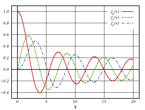
Today we will investigate how accurately MATLAB computes Bessel functions of the first and second kind Yn(x) and Jn(x) in double precision. Along the way, we will also check accuracy of the commonly used open source libraries.
Having extended precision routines, accuracy check of any function needs only few commands:
% Check accuracy of sine using 1M random points on (0, 16]
>> mp.Digits(34);
>> x = 16*(rand(1000000,1));

>> f = sin(x);       % call built-in function for double precision sine
>> y = sin(mp(x));   % compute sine values in quadruple precision
>> z = abs(1-f./y);  % element-wise relative error

>> max(z./eps)       % max. relative error in terms of 'eps'
ans =
    0.5682267303295349594044472141263213

>> -log10(max(z))    % number of correct decimal digits in result
ans =
    15.89903811472552788729580391380739
Computed sine values have ~15.9 correct decimal places and differ from ‘true’ function values by ~0.5eps. This is the highest accuracy we can expect from double precision floating-point arithmetic.
The recent revision of IEEE 754 standard[1] recommends all elementary functions to have such highest accuracy and be correctly rounded: the result should be as if the calculation had been performed in infinite precision, and then rounded (see Table 9.1 of the standard). Computing elementary functions with correct rounding is a fascinating topic on its own, please refer to pioneering works of Gal[2, 3], Ziv[4], recent developments by Lefèvre, Muller, Zimmermann, et al.[5–8] and excellent handbooks on the subject[9–11].
Most modern programming languages follow the IEEE 754-2008 recommendation and their standard libraries[12,13,14] compute elementary functions with correct rounding and guaranteed accuracy as we see in test above.
However special functions are not covered by the standard and software libraries for its computations are considered to be faithfully-accurate. Here we study what libraries in fact can be trusted in computing Bessel functions in double precision.
MATLAB 2016a
Basic accuracy check applied for Bessel function of the second kind – Y0(x):
% Check accuracy of bessely(0,x) using 1M random points on (0, 16]
>> f = bessely(0,x);     % built-in double precision routine
>> y = bessely(0,mp(x)); % 'true' values computed using quadruple precision
>> z = abs(1-f./y);

>> max(z./eps)           % max. relative error in terms of 'eps'
ans =
    1366834.014340578752744356956505545

>> -log10(max(z))        % number of correct decimal digits in result
ans =
    9.517843996632803435430170368588769
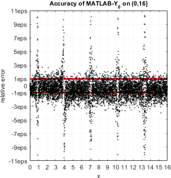
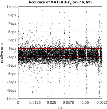
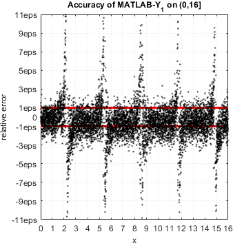
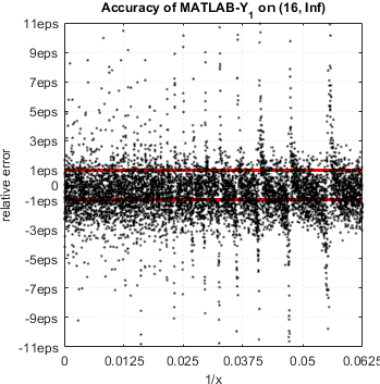
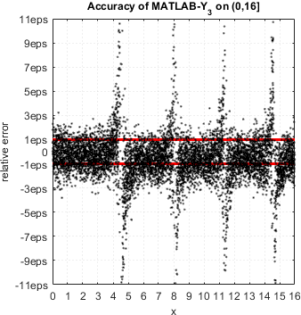
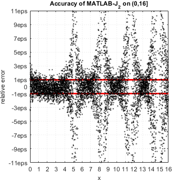
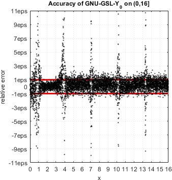
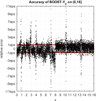
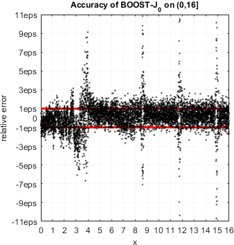
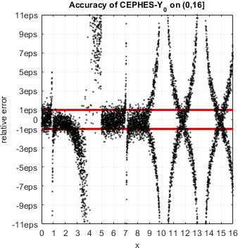
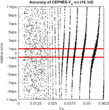
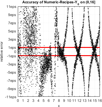
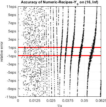
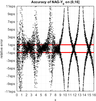
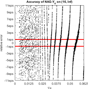
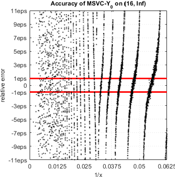
The problematic areas can be located using error scatter plot. Red lines show the expected limits of relative error (for convenience, we added another interval to cover whole x axis):
The spikes of error clearly coincide with zeros of Bessel function (0.8935, 3.9576, 7.0860, ... ). To test accuracy near zeros in more detail we use the following function:
function func_accuracy_check(func, x0, near_zero, n)
%func_accuracy_check - Checks accuracy of 'func' near its zero or extremum.
%
%  1. Routine searches for zero/extremum of 'func' starting from 'x0'
%     Extended precision is used to be sure zero/extremum is accurate.
%
%  2. Relative error of 'func' is evaluated using 'n' points in close
%     vicinity of found zero/extremum.
%
%  Parameters:
%   func - function handle
%   x0 - starting point for zero/extremum search
%   near_zero - true/false, check accuracy near zero/extremum
%   n - number of test points.
%
%  Usage example.
%    Find zero of Y0(x) near x = 2 and check accuracy of the MATLAB
%    function bessely(0,x) near found zero:
%
%    mp.Digits(34);
%    u = @(x) bessely(0,x);
%    func_accuracy_check(u,mp(2),true,3)
%
%    Output:
%    Accuracy check near zero, x = 8.9357696627916752e-01:
%    x = 8.9357696627916761e-01	correct digits =   1.5	rel. error = 1.40e+14eps
%    x = 8.9357696627916772e-01	correct digits =   0.5	rel. error = 1.50e+15eps
%    x = 8.9357696627916783e-01	correct digits =   1.0	rel. error = 4.13e+14eps

% Find root/extremum of 'func' using extended precision:
options = optimset('TolX',mp('eps'));
if near_zero
    r = fzero(func,mp(x0),options);
    fprintf('Accuracy check near zero, x = %.16e:\n',r);
else
    %g = @(x) -func(x);
    r = fminsearch(func,mp(x0),options);
    fprintf('Accuracy check near extremum, x = %.16e:\n',r);
end;

% Correctly rounded zero/extremum in double precision:
x = double(r);
for k=1:n
    % Get next floating-point value after x:
    x = nextafter(x);

    f = func(x);      % function value computed by MATLAB's built-in bessely
    y = func(mp(x));  % 'true' function value computed in extended precision

    z = abs(1-f./y);  % relative accuracy
    fprintf('x = %.16e\tcorrect digits = %4.1f\trel. error = %5.2geps\n',x,-log10(z),z./eps);
end
The nextafter(x) function computes next floating-point value just after x[15] towards infinity. We use it to generate test arguments in close neighborhood of given point.
Accuracy of bessely(0,x) near first zero of Y0(x):
>> mp.Digits(34);
>> u = @(x) bessely(0,x);
>> func_accuracy_check(u,mp(2),true,5)
Accuracy check near zero, x = 8.9357696627916752e-01:
x = 8.9357696627916761e-01  correct digits =  1.5  rel. error = 1.4e+14eps
x = 8.9357696627916772e-01  correct digits =  0.5  rel. error = 1.5e+15eps
x = 8.9357696627916783e-01  correct digits =  1.0  rel. error = 4.1e+14eps
x = 8.9357696627916794e-01  correct digits =  2.1  rel. error = 3.5e+13eps
x = 8.9357696627916805e-01  correct digits =  1.4  rel. error = 1.6e+14eps
Accuracy of bessely(0,x) near second extremum of Y0(x):
>> func_accuracy_check(u,mp(3),false,5)
Accuracy check near extremum, x = 5.4296810407941351e+00:
x = 5.4296810407941356e+00  correct digits = 15.6  rel. error =  1.10eps
x = 5.4296810407941365e+00  correct digits = 16.2  rel. error =  0.32eps
x = 5.4296810407941374e+00  correct digits = 16.0  rel. error =  0.42eps
x = 5.4296810407941383e+00  correct digits = 16.0  rel. error =  0.42eps
x = 5.4296810407941392e+00  correct digits = 15.6  rel. error =  1.10eps
MATLAB delivers minimal error near extremum but completely losses accuracy near function zero.
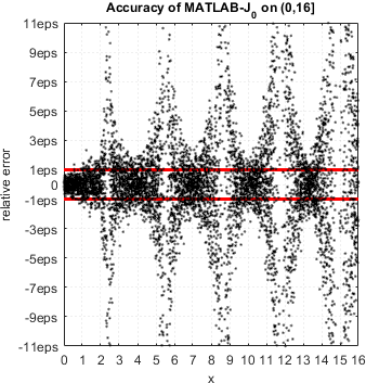
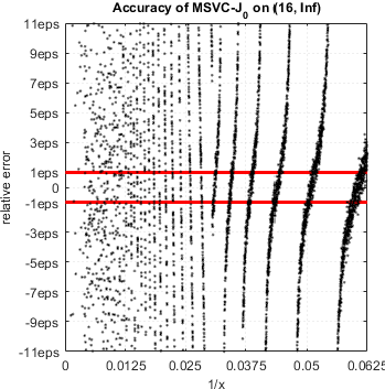
Same analysis can be easily repeated for J0(x):
Accuracy of besselj(0,x) near first zero of J0(x):
>> u = @(x) besselj(0,x);
>> func_accuracy_check(u,mp(2),true,5)
Accuracy check near zero, x = 2.4048255576957728e+00:
x = 2.4048255576957733e+00  correct digits =  0.6  rel. error = 1.2e+15eps
x = 2.4048255576957738e+00  correct digits =  1.0  rel. error = 4.7e+14eps
x = 2.4048255576957742e+00  correct digits =  0.8  rel. error = 7.4e+14eps
x = 2.4048255576957747e+00  correct digits =  1.9  rel. error = 5.9e+13eps
x = 2.4048255576957751e+00  correct digits =  1.4  rel. error = 1.6e+14eps
Accuracy of besselj(0,x) near first extremum of J0(x):
>> func_accuracy_check(u,mp(2),false,5)
Accuracy check near extremum, x = 3.8317059702075123e+00:
x = 3.8317059702075129e+00  correct digits = 15.8  rel. error =  0.71eps
x = 3.8317059702075134e+00  correct digits = 15.8  rel. error =  0.71eps
x = 3.8317059702075138e+00  correct digits = 15.5  rel. error =  1.30eps
x = 3.8317059702075142e+00  correct digits = 15.8  rel. error =  0.71eps
x = 3.8317059702075147e+00  correct digits = 15.9  rel. error =  0.53eps
Situation is the same – besselj(0,x) computes J0(x) incorrectly near zeros.
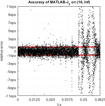
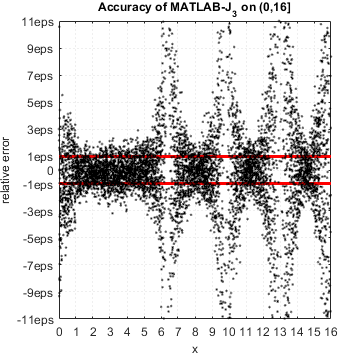
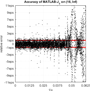
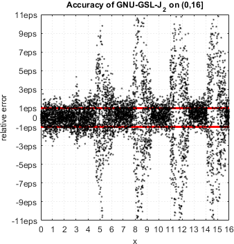
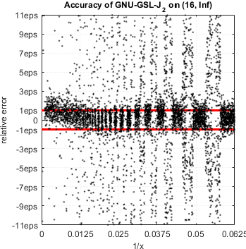
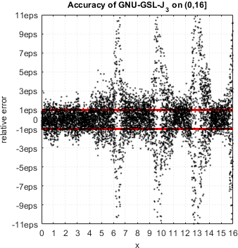
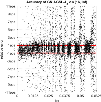
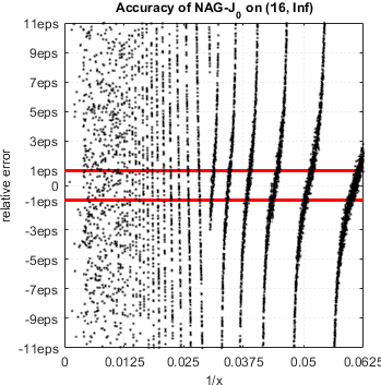
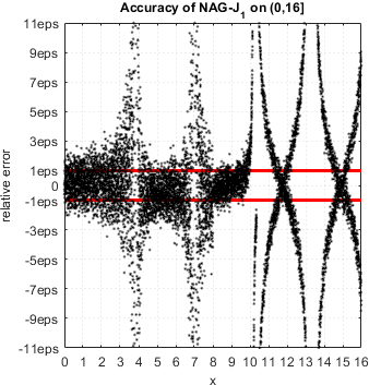
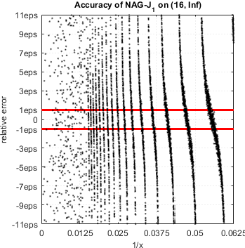
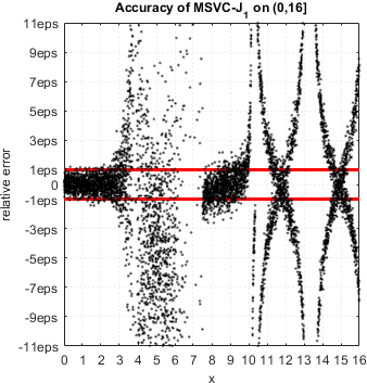
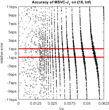
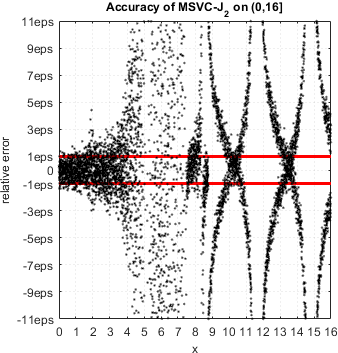
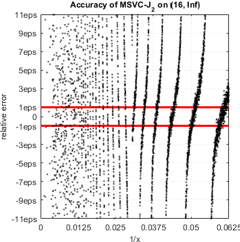
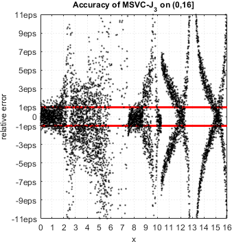
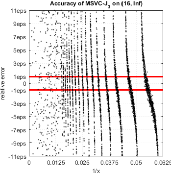
In fact, all routines in MATLAB for computing Bessel functions of integer order suffer from accuracy loss in vicinity of function zeros. Error can be arbitrary high, even to the point when none of the digits are correct.
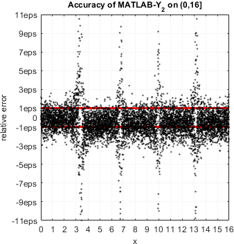
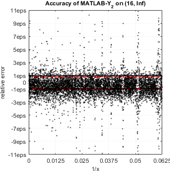
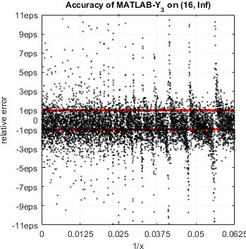
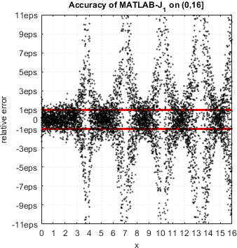
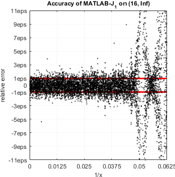
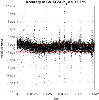
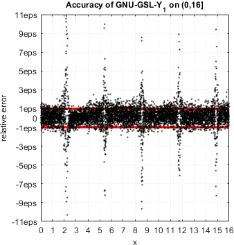
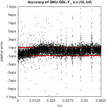
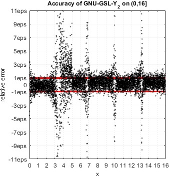
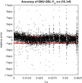
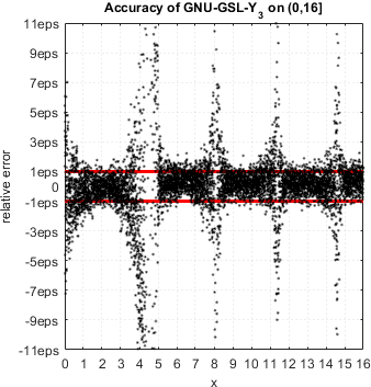
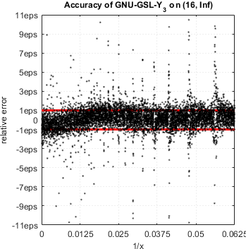
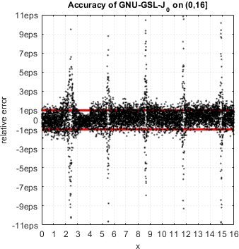
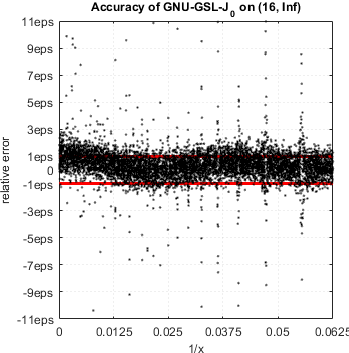
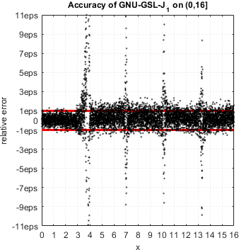
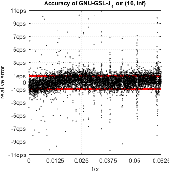
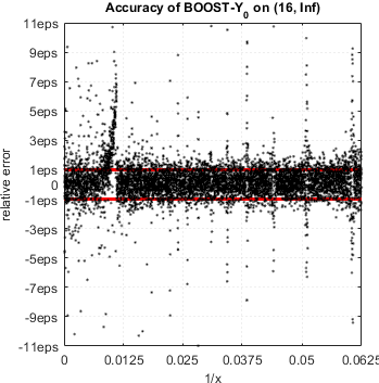
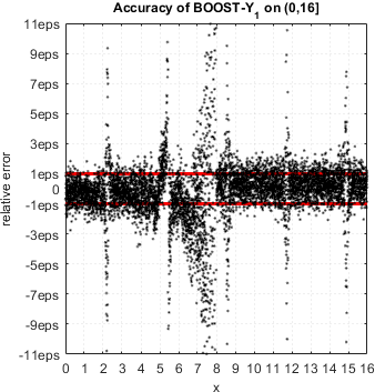
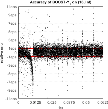
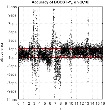
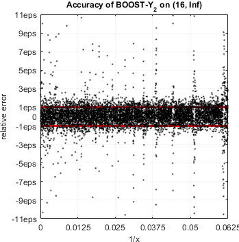
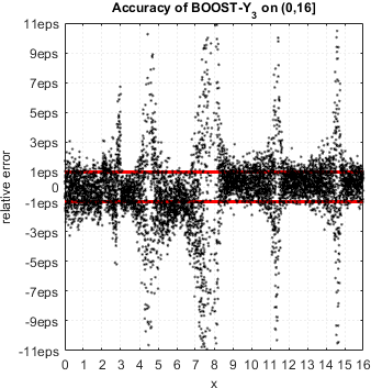
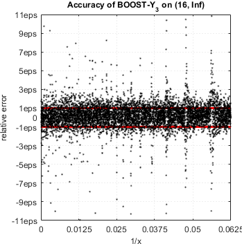
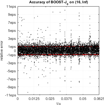
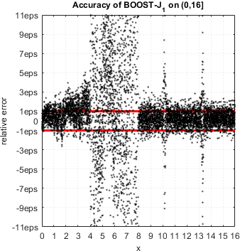
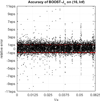
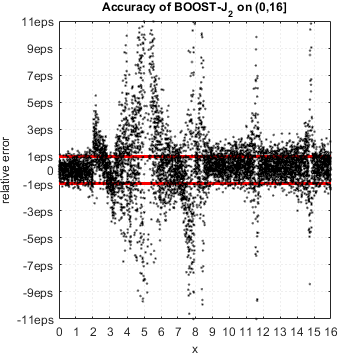
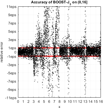
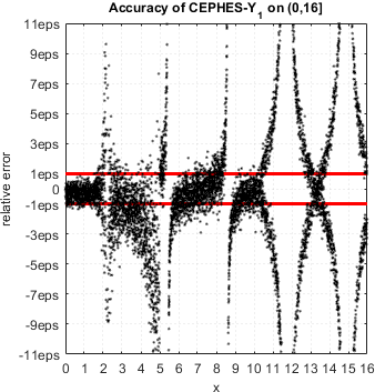
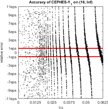
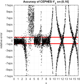
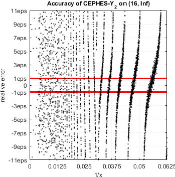
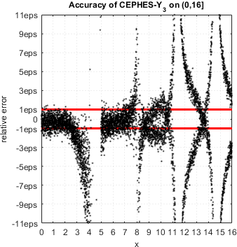
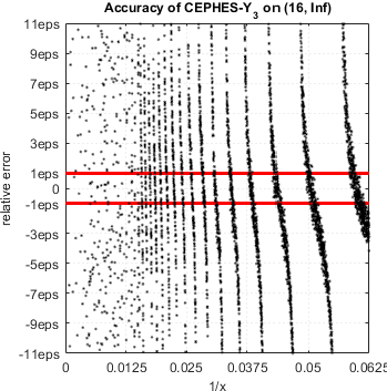
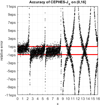
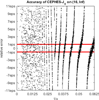
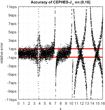
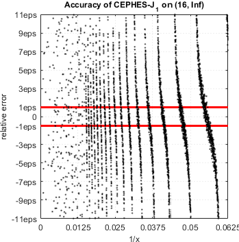
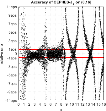
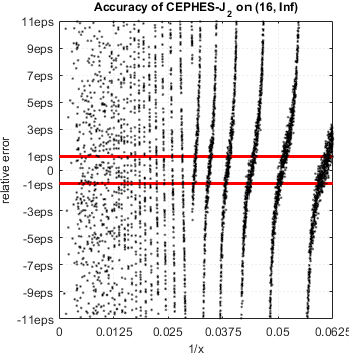
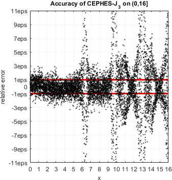
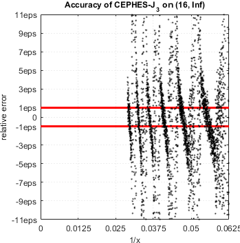
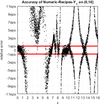
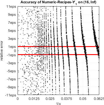
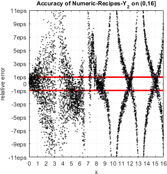
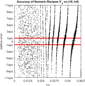
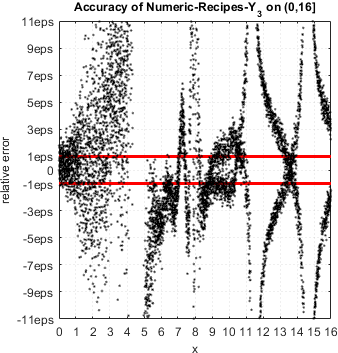
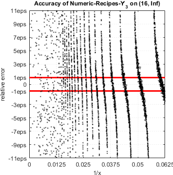
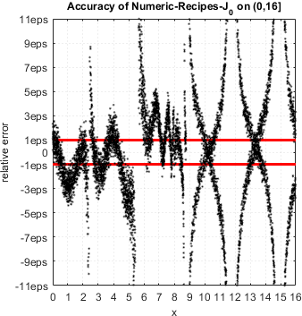
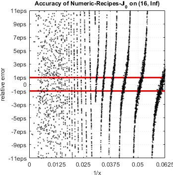
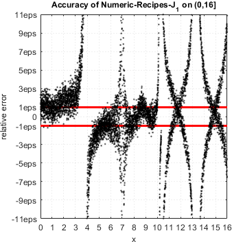
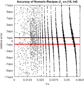
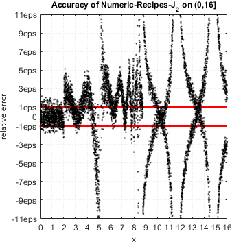
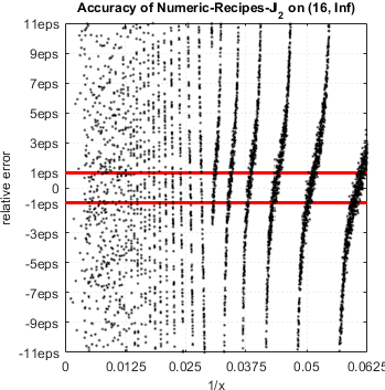
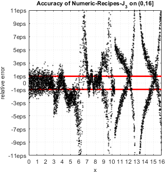
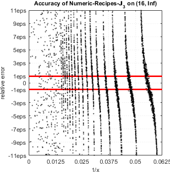
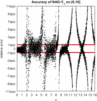
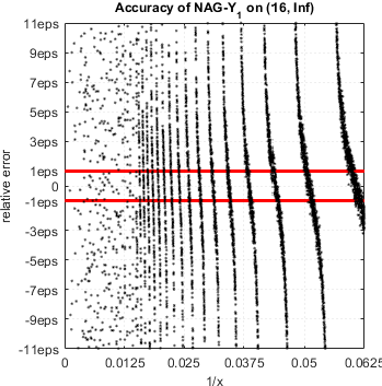
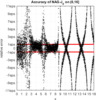
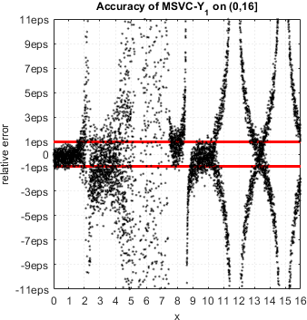
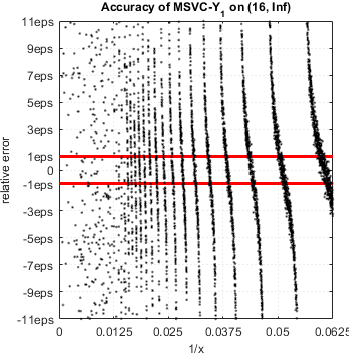
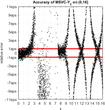
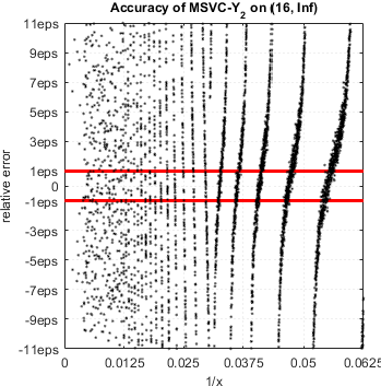
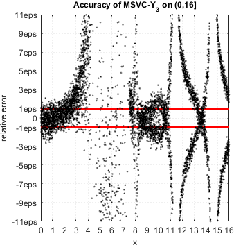
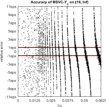
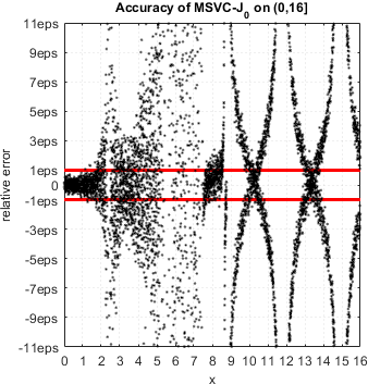
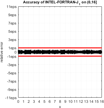
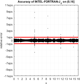
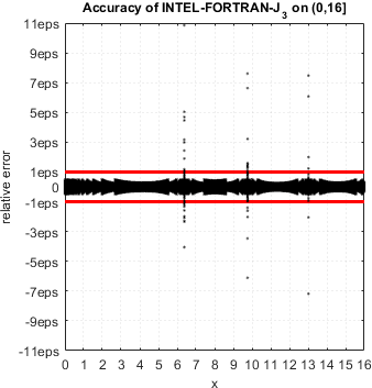
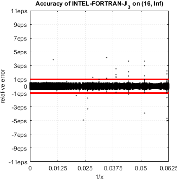
Below we just show relative error plots with obvious peaks near function zeros – indication of accuracy loss (detailed analysis for every function can be easily done using routine above):
Certainly this situation is absolutely unacceptable, and TMW should re-consider its library for computing Bessel functions.
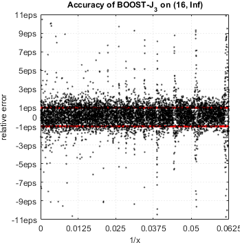
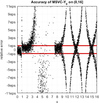
More surprisingly, the issue is endemic for nearly all libraries for computing Bessel functions in double precision! Below we present error plots for some commonly used open source and commercial libraries. All of them (except one) suffer from the same accuracy loss near function zeros – error may become arbitrary high.
Part of several generations of MS Visual Studio [21]
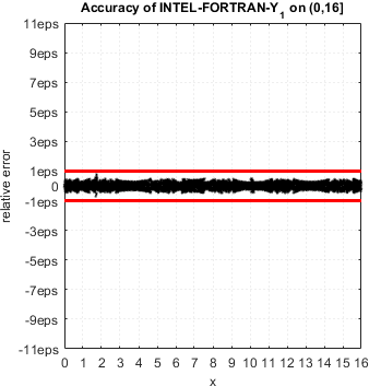
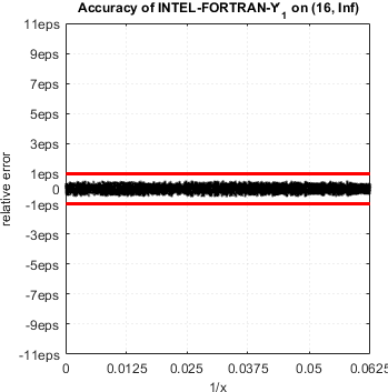
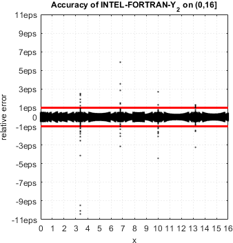
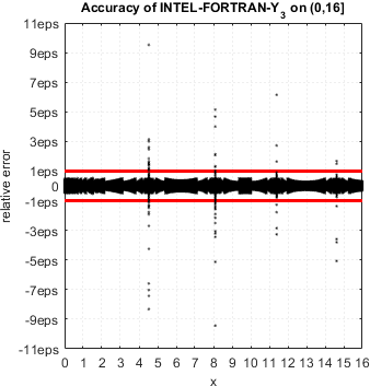
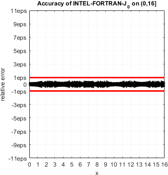
Intel Fortran
Conclusion
All tested commercial (MATLAB, NAG, Intel and Microsoft) and open source libraries (GNU GSL, Boost, CEPHES and Numeric Recipes) exhibit severe accuracy degradation near zeros of Bessel functions. In fact, computed function values have no correct digits in close vicinity of zeros.
Intel mathematical library delivers accurate results for Y0(x), Y1(x), J0(x) and J1(x) but suffers from the same accuracy loss for higher orders n=2,3,....
The difficulty of approximating Bessel functions near zeros is well known[22] and efficient algorithms were developed for both cases – double[23] and arbitrary precision[24]. We hope maintainers of the libraries will take this analysis into account and will provide fixes in future releases.
Until then, please rely on high-accuracy tools, e.g. Advanpix toolbox which is the only way to compute Bessels correctly in MATLAB at the moment.
S. Gal. Computing elementary functions: A new approach for achieving high accuracy and good performance. In Accurate Scientific Computations. Lecture Notes in Computer Science, volume 235, pages 1–16. Springer-Verlag, Berlin, 1986.
S. Gal and B. Bachelis. An accurate elementary mathematical library for the IEEE floating point standard. ACM Transactions on Mathematical Software, 17(1):26–45, March 1991.
A. Ziv, Fast Evaluation of Elementary Mathematical Functions with Correctly Rounded Last Bit, ACM Trans. Math. Software, vol. 17, no. 3, pp. 410-423, 1991.
V. Lefevre and J.-M. Muller, Worst Cases for Correct Rounding of the Elementary Functions in Double Precision, Proc. 15th IEEE Symp. Computer Arithmetic (ARITH 15), N. Burgess and L. Ciminiera, eds., pp. 111-118, 2001
D. Defour, G. Hanrot, V. Lefevre, J.-M. Muller, N. Revol, and P. Zimmermann, Proposal for a Standardization of Mathematical Function Implementation in Floating-Point Arithmetic, Numerical Algorithms,vol. 37, nos. 1-4, pp. 367-375, 2004
D. Stehle and P. Zimmermann. Gal’s accurate tables method revisited. In Proceedings of the 17th IEEE Symposium on Computer Arithmetic (ARITH-17). IEEE Computer Society Press, Los Alamitos, CA, 2005.
Catherine Daramy-Loirat, David Defour, Florent de Dinechin, Matthieu Gallet, Nicolas Gast, and Jean-Michel Muller. CR-LIBM: A library of correctly rounded elementary functions in double-precision, February 29, 2009.
P. W. Markstein. IA-64 and Elementary Functions: Speed and Precision. Hewlett Packard Professional Books. Prentice Hall, 2000.
Press, William H. and Teukolsky, Saul A. and Vetterling, William T. and Flannery, Brian P. Numerical Recipes 3rd Edition: The Art of Scientific Computing, 2007, Cambridge University Press, New York, USA.
J. F. Hart, E. W. Cheney, C. L. Lawson, H. J. Maehly, C. K. Mesztenyi, J. R. Rice, H. G. Thatcher, and C. Witzgall. Computer Approximations. Robert E. Krieger, 1978.
J. Harrison. Fast and Accurate Bessel Function Computation, Proceedings of ARITH19, the 19th IEEE Conference on Computer Arithmetic, IEEE Computer Society Press, 2009, pp. 104-113.
Absolutely amazing work! This is a serious issue, that I run into with my students, when expanding functions in a Bessel series. I can’t tell you how often I have said “yes, that looks sh*t because Matlab’s Bessel function are sh*t. We have to stop after a few terms in the series”.
external function usage may need change, see following example we met when use IVF19 (don’t need declare) to compile old code works on IVF9 (need declare)
Remove MSTA1, MSTA2 declare in INT statement solved the problem
For this method you will need to access your WordPress site’s root folder by using FTP or File Manager app in your hosting account’s cPanel dashboard.
In most cases if you are on a shared host, then you will not see a php.ini file in your directory. If you do not see one, then create a file called php.ini and upload it in the root folder. In that file add the following code: