Uncategorised

If you’ve built agent workflows with pure prompting, you’ve likely run into hard limits. The model can generate logic, but it cannot securely execute code, call authenticated APIs, persist state, or orchestrate multi-step tool chains on its own.

Claude Code Skills provides that missing execution layer. They let Claude interface with external systems, manage authentication, query databases, automate browser operations, and maintain structured context across sessions. You move from simulated workflows to real system interactions.

For developers and teams building production-grade AI agents, skills define what the system can actually do.

Here are the top 10 Claude Code skills that matter.

TL;DR

• Claude Code Skills extends Claude with modular execution capabilities such as tool access, sandboxed code, memory, and structured workflows.
• Composio — serves as the integration backbone with 850+ SaaS apps, OAuth lifecycle management, scoped credentials, and standardized action schemas.
• Remotion Best Practices — gives Claude deep knowledge of animations, timing, audio, captions, and 3D so it writes correct Remotion code every time
• Frontend Design — forces a bold design direction upfront — brutalist, maximalist, retro-futuristic, whatever — then executes with precision instead of defaulting to generic AI slop
• agent-browser — lets Claude control any web interface through stable element refs, no clean API required, with full support for clicks, fills, screenshots, and parallel sessions
• Supermemory — tracks facts about users over time, handles contradictions, auto-forgets expired info, and delivers personalized context in under 50ms
• File/Document Processing — gives Claude direct access to PDFs, spreadsheets, and CSVs for parsing, cleaning, validating, and converting into pipeline-ready formats
• Marketing Skills — packages marketing strategy, campaign planning, and content creation into repeatable workflows instead of one-off prompt chains
• agent-sandbox-skill — spins up isolated cloud sandboxes where Claude can build, host, and test full-stack apps without ever touching your local files or production environment
• Superpowers — walks the agent through brainstorm → spec → plan → subagent execution → review → merge, keeping multi-step dev work structured and on track
• Web Design Guidelines — pulls the latest design rules from the source repo and checks your interface code against every one of them before you ship

What Are Claude Code Skills?

Claude Code Skills package execution logic into structured, reusable modules that extend an agent’s capabilities. They move workflow logic out of oversized prompts and into versioned units you can inspect, update, and reuse.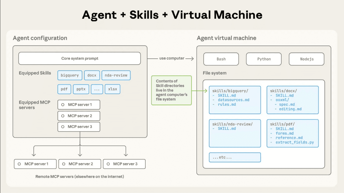

A skill defines how Claude should perform a specific class of tasks. Inside a skill, you can include:

• Metadata for discovery
• Explicit operational steps
• Domain constraints
• Supporting reference files
• Executable scripts

This structure lets you codify repeatable workflows once and apply them consistently. You reduce prompt sprawl, cut token overhead, and gain tighter control over the agent’s behaviour.

When you build with skills, you stop embedding fragile logic in long prompts. You encapsulate behaviour into clear modules and let Claude load them when needed.

Skill Architecture and Execution Model

Each skill lives in its own directory and starts with a SKILL.md file. That file defines the skill’s name, purpose, and step-by-step execution logic. Claude reads the metadata first to determine relevance. When the task matches, Claude loads the full instructions and any supporting files.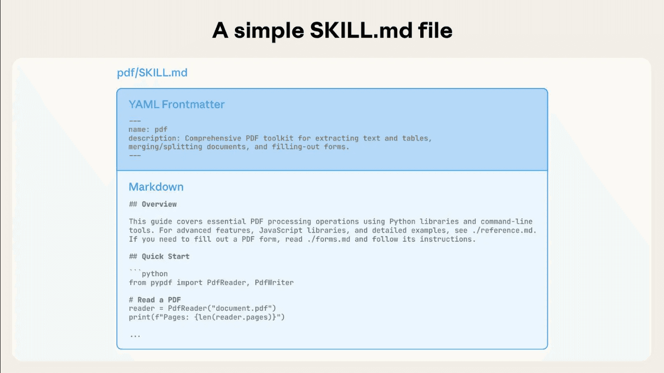

You can attach scripts to a skill and run them in a sandbox. Claude can execute deterministic logic, call APIs, process files, and manage multi-step workflows reliably.

Claude combines skills on a task basis, so you can build complex workflows without bloated prompts. This modular setup keeps execution structured and easier to scale.

Top 10 Claude Code Skills for Production Grade Agents

These skills consistently appear in real-world builds. They cover infrastructure, execution, data access, and orchestration. These layers move agents from demo to deployment.

Let us now look at the 10 Claude Code skills teams rely on to build and ship production-grade agents.

1. Composio Skills

Composio functions as an agent-native integration and execution layer. It standardizes external APIs into structured, callable tools that Claude can discover and invoke through a consistent schema.

You register integrations once and expose them as normalized tool interfaces. The agent selects tools dynamically based on task context and passes structured arguments that map directly to validated API operations.

Add Composio skills to your AI assistant:

This command installs the Composio agent skills, giving your AI assistant access to:

• Tool Router best practices – Session management, authentication, and framework integration
• Triggers & Events – Real-time webhooks and event handling
• Production patterns – Security, error handling, and deployment guides

Your AI assistant can now reference these skills when helping you build with Composio!

Technical capabilities include:

• 1000+ prebuilt toolkits mapped to typed action schemas
• OAuth 2.0 and API key lifecycle management with automatic token refresh
• Scoped credential isolation per agent, environment, or workflow
• Tool discovery via metadata indexing and semantic matching
• Deterministic request construction with validated input parameters
• Structured JSON responses for downstream chaining
• Sandboxed execution environment for safe tool invocation
• Execution logs, traceability, and observability for debugging

Composio abstracts API heterogeneity into a uniform execution layer. Claude emits structured tool calls, and Composio validates, authenticates, executes, and returns machine-readable outputs.

Repo: https://github.com/ComposioHQ/skills | Docs: https://docs.composio.dev

2. Remotion Best Practices Skill

The Remotion Best Practices Skill gives Claude deep domain knowledge for building programmatic videos with React. It loads specialized rules for animations, timing, audio, captions, 3D, and more — ensuring Claude generates correct, idiomatic Remotion code every time.

Install it with:

This skill covers:

• Animations & timing — interpolation curves, spring animations, easing, sequencing, and transitions
• Audio & captions — importing audio, trimming, volume control, subtitles via Mediabunny
• Media handling — videos, images, GIFs, Lottie, fonts, and transparent video rendering
• 3D content — Three.js and React Three Fiber integration inside Remotion compositions
• Charts & data viz — bar, pie, line, and stock chart patterns
• Advanced patterns — dynamic metadata, parametrizable videos with Zod schemas, Mapbox maps, ElevenLabs voiceover

With 117K+ weekly installs and security audits from Agent Trust Hub and Socket, it is one of the most widely used official skills in the ecosystem. It activates automatically whenever Claude is working with Remotion code, loading only the relevant rule files on demand to stay context-efficient.

Skill repo: github.com/remotion-dev/skills | Full reference: skills.sh/remotion-dev/skills/remotion-best-practices

3. Frontend Design Skill

The Frontend Design Skill guides Claude to create distinctive, production-grade interfaces that avoid generic “AI slop” aesthetics. Before writing a single line of code, it pushes Claude to commit to a bold conceptual direction — brutally minimal, maximalist chaos, retro-futuristic, art deco, editorial, and more — then execute it with full precision.

Install it with:

This skill enforces:

• Typography — distinctive display/body font pairings; never generic choices like Inter, Roboto, or Arial
• Color & theme — cohesive CSS variable systems with dominant colors and sharp accents over timid palettes
• Motion — high-impact animations, staggered reveals, scroll-triggered effects, and meaningful hover states
• Spatial composition — asymmetry, overlap, diagonal flow, grid-breaking elements, and intentional negative space
• Backgrounds & depth — gradient meshes, noise textures, geometric patterns, layered transparencies, and grain overlays

The skill works across HTML/CSS/JS, React, and Vue, and scales implementation complexity to match the aesthetic vision — maximalist designs get elaborate animations, minimalist designs get precision spacing and restraint. With 110K+ weekly installs across Claude Code, Codex, Gemini CLI, and GitHub Copilot, it is one of the most widely adopted design skills in the ecosystem.

Skill repo: github.com/anthropics/skills | Full reference: skills.sh/anthropics/skills/frontend-design

4. Browser Automation Skill (agent-browser)

agent-browser is a headless browser automation CLI from Vercel Labs, purpose-built for AI agents. It pairs a fast Rust binary with a Node.js/Playwright daemon, giving Claude deterministic, ref-based control over any web interface without needing clean APIs.

Install it with:

The optimal AI workflow is snapshot-first:

Key capabilities:

• Ref-based selection — snapshot returns stable @e1, @e2 refs for deterministic, AI-friendly element targeting
• Full interaction suite — click, fill, drag, upload, hover, scroll, dialogs, frames, tabs, and keyboard/mouse control
• Network control — intercept, mock, and block requests; set headers scoped to origin for auth without login flows
• Isolated sessions & profiles — run multiple parallel browser instances with persistent cookie/auth state
• Live streaming — WebSocket viewport stream for pair browsing alongside an agent
• Cloud providers — swap local Chromium for Browserbase, Browser Use, or Kernel with a single flag
• iOS Simulator — control real Mobile Safari via Appium for authentic mobile web testing

With 14K GitHub stars and skills support for Claude Code, Cursor, Codex, Gemini CLI, and Copilot, agent-browser is the production-grade choice for agentic web automation.

Repo: github.com/vercel-labs/agent-browser | Docs: agent-browser.dev

5. Memory and Context Management Skill (Supermemory)

Supermemory is the #1-ranked memory and context engine for AI — topping LongMemEval, LoCoMo, and ConvoMem, the three major AI memory benchmarks. Unlike RAG (which retrieves static document chunks), Supermemory extracts and tracks facts about users over time, understands temporal changes, resolves contradictions, and automatically forgets expired information.

Install the Claude Code plugin:

Once installed, your agent gets three tools that fire automatically:

• memory — saves or forgets information; called automatically when you share something worth remembering
• recall — searches memories by query and returns relevant results alongside your user profile summary
• context — injects your full profile (preferences, recent activity) into the conversation at the start of each session; in Claude Code, just type /context

The full context stack in one API:

• Memory Engine — extracts facts from conversations, tracks updates, resolves contradictions, auto-forgets expired info
• User Profiles — auto-maintained per-user context (static facts + recent dynamic activity) delivered in ~50ms
• Hybrid Search — RAG + Memory in a single query; returns knowledge base docs and personalized context together
• Connectors — real-time sync from Google Drive, Gmail, Notion, OneDrive, GitHub via webhooks
• Multi-modal Extractors — PDFs, images (OCR), videos (transcription), code (AST-aware chunking)

Integrates as a drop-in wrapper with Vercel AI SDK, LangChain, LangGraph, OpenAI Agents SDK, Mastra, and Agno. With 16.7K GitHub stars and benchmarks proving state-of-the-art recall, it’s the most production-proven memory layer in the ecosystem.

Repo: github.com/supermemoryai/supermemory | Docs: supermemory.ai/docs

1. File System and Document Processing Skill

The File System and Document Processing Skill gives Claude controlled access to file environments, enabling direct work with PDFs, spreadsheets, CSVs, and structured reports in enterprise workflows.

Install it with:

Key capabilities:

• PDF extraction — parse tables, text blocks, and metadata from complex documents
• Spreadsheet normalization — clean, validate, and transform Excel/CSV data into structured formats
• Field validation — enforce schemas, detect anomalies, and flag inconsistencies in structured data
• Format conversion — transform raw files into JSON, XML, or database-ready outputs
• Batch processing — handle multiple documents in parallel with consistent transformation rules

The skill operates on actual file contents, producing verifiable outputs that integrate seamlessly with databases, analytics pipelines, and workflow engines. Document-heavy operations become programmable components inside broader automation systems rather than isolated manual tasks.

Repo: github.com/ComposioHQ/awesome-claude-skills

7. Marketing Skills (marketingskills)

The Marketing Skills package provides Claude with specialized knowledge for marketing strategy, campaign execution, and content creation. It helps the agent generate marketing materials, analyze campaigns, and implement best practices across various marketing channels.

Install it with:

This skill enables Claude to assist with marketing workflows, content strategy, campaign planning, and performance analysis — turning marketing tasks into structured, repeatable operations that integrate with broader automation systems.

Repo: github.com/coreyhaines31/marketingskills

8. Code Execution Sandbox Skill (agent-sandbox-skill)

agent-sandbox-skill gives Claude (and other coding agents) a fully isolated E2B cloud sandbox to plan, build, host, and test full-stack applications — all without touching your local filesystem or production environment. Each agent fork gets its own independent sandbox, making it safe to run untrusted code, install packages, or spin up servers at any scale.

The core workflow is a single command:

This orchestrates a full Plan → Build → Host → Test lifecycle. Individual commands are also available for finer control:

• \sandbox <prompt> — ad-hoc sandbox operations with minimal compute
• \agent-sandboxes:plan-full-stack <prompt> — generates a detailed implementation plan with browser UI testing workflows
• \agent-sandboxes:build <plan_path> — executes a build plan inside the sandbox
• \agent-sandboxes:host <sandbox_id> <port> — exposes a port and returns a public URL
• \agent-sandboxes:test — runs validation tests including browser UI testing via built-in Playwright integration

Key capabilities:

• Isolation — every agent fork runs in a gated E2B sandbox, fully separated from local files and production systems
• Scale — run as many parallel sandboxes as needed; each is independent with its own compute
• Full-stack development — scaffold, build, and host Vue + FastAPI + SQLite apps end-to-end
• Persistent context — tools to manage sandbox lifecycles across agent turns
• Prompt library — 40+ tiered prompts (very easy → very hard) for real full-stack app workflows, tested with Claude Sonnet, Opus 4.5, Gemini, and Codex

Setup requires Python 3.12+, uv, and an E2B API key. Works with Claude Code, Gemini CLI, and Codex CLI out of the box.

Repo: github.com/disler/agent-sandbox-skill | E2B docs: e2b.dev/docs

9. Multi-Agent Orchestration Skill (Superpowers)

Superpowers is a complete agentic software development workflow built on a composable skills framework. Rather than jumping straight into code, it guides the agent through a structured process: brainstorm → design spec → implementation plan → subagent-driven execution → review → merge.

Install in Claude Code via the plugin marketplace:

The core workflow steps:

• brainstorming — refines rough ideas through Socratic questions, presents the design in digestible chunks for sign-off, saves a design document
• using-git-worktrees — creates an isolated branch and workspace after design approval, verifies a clean test baseline before any code is written
• writing-plans — breaks approved designs into 2–5 minute tasks with exact file paths, complete code, and verification steps
• subagent-driven-development — dispatches a fresh subagent per task with two-stage review (spec compliance, then code quality); Claude can often run autonomously for hours without deviating
• test-driven-development — enforces strict RED-GREEN-REFACTOR; deletes any code written before a failing test exists
• requesting-code-review + finishing-a-development-branch — reviews against plan by severity, then presents merge/PR/keep/discard options and cleans up the worktree

Skills trigger automatically — the agent checks for relevant skills before any task, making the entire workflow mandatory rather than optional. With 40.9K GitHub stars and 3.1K forks, Superpowers is the most battle-tested multi-agent development methodology in the ecosystem.

Repo: github.com/obra/superpowers | Marketplace: github.com/obra/superpowers-marketplace

10. Web Design Guidelines Skill

The Web Design Guidelines Skill gives Claude the ability to review web interface code for compliance with established design standards. It fetches the latest guidelines from a canonical source and validates files against all defined rules, outputting findings in a structured format.

Install it with:

Key capabilities:

• Automatic guideline sync — fetches the latest rules from the source repository before each review
• File pattern matching — reviews specified files or prompts for file patterns to analyze
• Comprehensive rule checking — validates against all rules defined in the fetched guidelines
• Structured output — reports findings in terse file:line format for easy integration with development workflows
• Fresh validation — always uses the most current version of the guidelines, ensuring consistency with evolving standards

The skill operates by fetching guidelines from github.com/vercel-labs/web-interface-guidelines, reading the target files, applying all rules, and outputting violations. With 22K GitHub stars and 133.4K weekly installs across Claude Code, Cursor, Codex, Gemini CLI, and Copilot, it’s a widely adopted standard for web interface validation.

Repo: github.com/vercel-labs/agent-skills

Skills Best Practices

Writing Effective Skills

A well-written skill is a specific, focused instruction set — not a general-purpose prompt. Treat each skill like a module: it should do one thing well and compose cleanly with others.

• Start with a clear trigger condition. The skill should specify exactly when it activates — e.g. “before writing any code” or “when the user asks to deploy.” Vague triggers cause skills to fire too broadly or not at all.
• Use imperative language. Write instructions as direct commands: “Always run tests before committing”, not “You might want to consider running tests.” Agents follow directives more reliably than suggestions.
• Keep skills short and scannable. Long skills dilute attention. If a skill exceeds ~50 lines, split it into two focused skills with clear separation of concerns.
• Include examples of correct and incorrect behavior. Concrete examples reduce ambiguity and dramatically improve consistency, especially for edge cases.
• Version your skills. Treat SKILL.md like code — commit changes, document why you changed behavior, and roll back when a change degrades agent performance.

Combining Multiple Skills

The real power of skills comes from composition. Individual skills handle one concern; stacked together, they form a complete agentic workflow.

• Design for independence first. Each skill should be useful on its own before you compose it. Skills with tight dependencies on other skills create fragile systems that break when one piece changes.
• Establish a clear execution order. If skills have sequencing requirements (e.g. brainstorm before plan, plan before execute), make the order explicit in a top-level orchestration skill rather than burying it in each individual skill.
• Avoid conflicting instructions. When combining skills from different sources, audit for contradictions — e.g. one skill saying “always ask before running commands” and another saying “execute autonomously.” The agent will resolve conflicts inconsistently.
• Use a meta-skill to load context. A lightweight “project setup” skill that runs at session start can inject the right combination of skills for the current task, reducing the need to manually specify which skills apply.

Performance & Token Efficiency

Every skill adds tokens to your context window. At scale, bloated skill sets slow responses, increase costs, and dilute the model’s attention on the actual task.

• Load skills on demand, not by default. Don’t add every skill to every session. Use conditional loading — only inject skills relevant to the current task type (coding, research, writing, etc.).
• Prefer structured formats over prose. Bullet points and numbered lists consume fewer tokens than paragraphs and are easier for the model to parse. Reformatting a 300-word skill as a 20-line checklist often produces equal or better results.
• Deduplicate shared instructions. If three skills all say “never modify production without approval”, consolidate that into a single shared constraint skill. Repetition wastes tokens without improving reliability.
• Benchmark skill impact. Measure response latency and output quality with and without each skill active. If a skill adds significant tokens but doesn’t meaningfully change behaviour, trim it or remove it entirely.

Security & Permissions

Skills that grant agents access to filesystems, APIs, browsers, or external services require careful scoping. The most capable agents are also the most dangerous if permissions are too broad.

• Follow least-privilege by default. Skills should request only the permissions actually needed. A web search skill doesn’t need filesystem access. A database skill doesn’t need shell execution. Scope each skill to its minimum viable permission set.
• Require confirmation for destructive actions. Any skill that can delete, overwrite, deploy, or send data externally should include an explicit human-in-the-loop checkpoint before proceeding. Never make irreversible actions fire automatically.
• Audit third-party skills before use. Skills from external repos can contain arbitrary instructions. Read SKILL.md files carefully before adding them to production agents — treat them like code dependencies, not just configuration.
• Isolate credentials from skill content. API keys, tokens, and secrets should never appear in SKILL.md files. Use environment variables or a secrets manager and reference them by name in skill instructions.
• Log and monitor skill-triggered actions. In production agents, every action taken under a skill’s instruction should be logged with the triggering skill, the action taken, and the result. Observability is the foundation of safe autonomous operation.

Conclusion

Claude Code Skills determines whether your agent can actually execute inside real systems. Reasoning matters, but secure access, controlled execution, and structured integrations define production readiness.

Strong architectures focus on modular capabilities, clear permission boundaries, and observable workflows. When execution stays structured and traceable, automation scales without becoming fragile.

Most production-grade agent stacks depend on a unified integration backbone that connects model decisions to authenticated system actions. Platforms like Composio provide that core layer and enable agents to operate reliably across tools and environments.

Top 10 Claude Code Skills Every Builder Should Know in 2026ContentsMar 4, 2026

• TL;DR
• What Are Claude Code Skills?
• Top 10 Claude Code Skills for Production Grade Agents
• Skills Best Practices
• Conclusion

AuthorAkash

ShareCopy linkPost

---

Your agents decide. We make it happen.

Effective safety culture depends not only on good policies, but on how consistently and transparently they are applied across institutions. As part of our ongoing work on research culture and EDI, we’ve launched SafetyVoice UK — an independent, sector-wide platform for laboratory users, researchers, and technical staff across UK Higher Education to share anonymised experiences of how safety policies are applied in practice. Safety is fundamental. But clear communication, appropriate documentation, and opportunities for dialogue are what make policies work well for everyone. When these elements are inconsistent, it can affect confidence, wellbeing, and the ability to work effectively. SafetyVoice UK is open to contributors from any UK HEI or research organisation. Using AI-assisted anonymisation, the platform identifies common themes across the sector while protecting individual contributors — supporting a more transparent, EDI-aligned approach to safety governance. We welcome colleagues across the sector to share their experiences or perspectives. 🔗 https://safetyvoice.org.uk/ #HigherEducation #LabSafety #EDI #SafetyCulture #ResearchCulture

@UUK (Universities UK), @USHA_HE (Universities Safety & Health Association), or @AdvanceHE

https://unsloth.ai/docs/basics/vision-fine-tuning#vision-data-collator

In COMSOL: h_top = 14.4, h_bot = 7.2 W/m²K are fixed constants from t=0. Full convective cooling is applied from the very first second.

In TS: h is recomputed every timestep from the Churchill & Chu correlation at T_mean:

T_mean = float(np.mean(T))   # starts at T_amb = 20°C
ht = calc_h_top(T_mean)      # → h ≈ 0 at t=0 !

At t=0, T_mean = T_amb, so ΔT = 0, Ra = 0, h = 0. TS starts with essentially zero convective cooling and only builds up h as the board heats. The full h=14.4 isn’t reached until T_mean ≈ 55°C (ΔT ≈ 35K above ambient).

So early in the transient:

Time	COMSOL h_top	TS h_top (approx)
t = 0 s	14.4 W/m²K	~0
t = 60 s	14.4 W/m²K	~5–8
t = 300 s	14.4 W/m²K	~11–13
SS	14.4 W/m²K	14.4

TS has far less cooling during the transient → rises faster and higher. At SS both converge to the same h, so SS temperatures should match closely. This matches exactly what the chart shows.

Simple fix: evaluate h at a representative ΔT from the start (e.g., use the current local temperature rather than T_mean, or initialise h at the SS value and let it update). The most direct fix to match the COMSOL setup would be to use fixed h values:

# Option: fix h to SS calibrated values (matches COMSOL setup)
ht = calc_h_top(T_AMB + 35.0)   # evaluate at design ΔT=35K, constant
hb = calc_h_bottom(T_AMB + 35.0)

Or keep temperature-dependent h but evaluate at a better representative temperature than T_mean.no, I want fix that in comsol, not in TS, teach me how to defin ht and hb in comsol as fucntion of position and temperature.

In COMSOL, you define h as an expression in T directly in the Heat Flux boundary condition. Here’s how:

---

Step 1 — Define parameters (Global Definitions > Parameters)

Name	Expression	Description
T_amb	293.15[K]	Ambient temperature
k_air	0.0271[W/(m*K)]	Air conductivity
nu_air	1.655e-5[m^2/s]	Kinematic viscosity
alpha_air	2.34e-5[m^2/s]	Thermal diffusivity
L_c	0.0292[m]	Characteristic length (A/P)
H_SCALE	1.76	Nu calibration multiplier

---

Step 2 — Define variables (Global Definitions > Variables)

dT_surf   = max(T - T_amb, 0.001[K])
T_film    = (T + T_amb) / 2
beta_air  = 1 / T_film
Ra        = 9.81[m/s^2] * beta_air * dT_surf * L_c^3 / (nu_air * alpha_air)
Nu_top    = if(Ra < 1e7, 0.54 * Ra^0.25, 0.15 * Ra^(1/3))
Nu_bot    = 0.27 * Ra^0.25
h_top_fn  = Nu_top * k_air / L_c * H_SCALE
h_bot_fn  = Nu_bot * k_air / L_c * H_SCALE

max(..., 0.001) avoids Ra=0 at t=0 when T=T_amb.

---

Step 3 — Apply to boundary conditions

Top surface — Heat Flux BC:

• Type: General inward heat flux
• Expression: h_top_fn * (T_amb - T)

Bottom surface — Heat Flux BC:

• Expression: h_bot_fn * (T_amb - T)

Alternatively, use the built-in “Convective heat flux” type and enter h_top_fn in the h field — COMSOL will evaluate it locally at each surface node’s current T automatically.

---

What this achieves

• At t=0: T=T_amb, dT≈0, Ra≈0, h≈0 (matches TS behaviour)
• At SS: Ra≈71,000, h_top≈14.4, h_bot≈7.2 W/m²K (matches calibrated values)
• COMSOL evaluates the expression locally per element at each timestep — better than TS which uses T_mean globally
• The transient h buildup will match TS more closely

Are our bodies really full of microplastics? Why a scientific ‘bombshell’ is a call for better methods, not a reason to dismiss the plastic crisis.

By Zengbo Wang, Bangor University

Over the past few years, a wave of alarming headlines has suggested that human bodies are rapidly becoming reservoirs for plastic pollution. High-profile studies have claimed to detect micro- and nanoplastics (MNPs) in human blood, placentas, arteries, testes, and even brain tissue.

However, a fierce debate has recently erupted within the scientific community, throwing many of these discoveries into doubt. Experts warn that several of these studies suffer from severe methodological flaws, leading to false positives and exaggerated concentrations. One chemist even described the doubts as a “bombshell” that forces us to re-evaluate what we actually know about microplastics in the body.

The false positive problem: When fat masquerades as plastic The primary challenge in measuring MNPs in human tissue is their microscopic size, which pushes the absolute limits of today’s analytical technology. A major flashpoint in this debate centres around a widely used technique called Py-GC-MS, which involves heating a sample until it vaporises to identify its molecular weight.

The problem? Human tissue is full of natural fats (lipids) that can produce chemical signals nearly identical to those of common plastics like polyethylene and PVC. This flaw was brutally highlighted in response to a widely publicised study claiming microplastic levels in human brains were rapidly rising. Critics pointed out that the human brain is approximately 60% fat, making it highly susceptible to false positives. One leading environmental analytical chemist bluntly labelled the brain study a “joke,” while others noted it is biologically implausible for particles of the reported size (3 to 30 micrometres) to cross into the bloodstream and organs in such massive volumes.

A world saturated in plastic: The contamination conundrum Beyond analytical misidentifications, researchers face an existential hurdle: we live in a world coated in plastic, making background contamination practically unavoidable.

Biological samples are extraordinarily vulnerable; medical operating theatres, where solid tissue samples are usually taken, are notoriously “full of plastic”. Critics argue that many studies—often led by medical professionals rather than specialised analytical chemists—failed to employ “standard good laboratory practices”. Crucial steps, such as running rigorous “blank” control samples to properly account for background contamination, were frequently overlooked in the rush to publish.

The call for a ‘forensic’ approach To ensure the integrity of future research, a coalition of over 30 international scientists, led by Imperial College London and the University of Queensland, has urgently called for the adoption of a “forensic science approach”.

Because no single measurement technique is perfect, this framework urges laboratories to combine multiple, independent testing methods on the exact same samples. By mirroring the rigorous standards of forensic laboratories—meticulously controlling contamination and clearly communicating confidence levels—scientists can ensure that early, suggestive data is no longer presented as definitive proof. As Professor Leon Barron of Imperial College London notes, “Finding ‘something’ in the human body is not the same as proving it is plastic, and certainly not the same as proving it is harmful”.

The political and public health stakes The stakes of getting this science right are incredibly high. Poor-quality evidence has fuelled public scaremongering, leading to predatory businesses offering unscientific, expensive treatments—sometimes costing up to £10,000—that falsely claim to “clean” microplastics from the blood.

Conversely, the petrochemical industry and lobbyists may seize upon these methodological debates to sow doubt about the broader harms of plastic pollution. Recognising the need for bulletproof data to inform policy, lawmakers in the United States have recently introduced bipartisan legislation such as the proposed Microplastics Safety Act and the Plastic Health Research Act to mandate and fund comprehensive federal research.

Science working exactly as it should What we are witnessing is not the debunking of the plastic crisis, but the vital, sometimes messy process of scientific self-correction. We know definitively that humans are exposed to MNPs daily through our environment, food, and water. Now, we must support the painstaking, rigorous work required to discover exactly how much plastic is inside us, and what it is doing to our health, so that society can take effective, evidence-based action.

References:

• Carrington, D. (2026). ‘A bombshell’: doubt cast on discovery of microplastics throughout human body. The Guardian.

• Packaging Europe. (2026). ‘Bombshell’ article casts doubt on studies of microplastics in the human body.

• Stewart, J. & O’Hare, R. (2026). Experts urge caution over microplastics in tissue claims and call for forensic approach to improve accuracy. Imperial College London News.

• The Acta Group. (2025). Microplastics in 2025: Regulatory Trends and Updates.

• Wikipedia Contributors. Microplastics and human health. Wikipedia, The Free Encyclopedia.

https://www.theguardian.com/environment/2026/jan/13/microplastics-human-body-doubt

in the folder of : ~/.openclaw/devices$

run following can list when the devices were created.

python3 – << ‘EOF’
import json, time
with open(“/home/jameszbw/.openclaw/devices/paired.json”) as f:
data = json.load(f)

for dev_id, dev in data.items():
last = dev[“tokens”][“operator”][“lastUsedAtMs”]
created = dev[“createdAtMs”]
print(f”\nDevice: {dev_id}”)
print(f” clientId: {dev[‘clientId’]}”)
print(f” mode: {dev[‘clientMode’]}”)
print(f” platform: {dev[‘platform’]}”)
print(f” created: {time.ctime(created/1000)}”)
print(f” last used: {time.ctime(last/1000)}”)
EOF

if openclaw veriosn mismatch gateway verison, use this:

openclaw gateway install –force

Agent-Capable LLM Comparison

In this table, we compare 2026’s leading open-source LLMs for agent workflows, each with a unique strength. For purpose-built agent applications, GLM-4.5-Air provides optimized tool use and web browsing. For specialized agentic coding, Qwen3-Coder-30B-A3B-Instruct delivers state-of-the-art performance. For complex reasoning agents, Qwen3-30B-A3B-Thinking-2507 offers advanced thinking capabilities. This side-by-side view helps you choose the right model for your specific agent workflow needs.

Number	Model	Developer	Subtype	SiliconFlow Pricing (Output)	Core Strength
1	GLM-4.5-Air	zai	Reasoning, MoE, 106B	$0.86/M tokens	Purpose-built agent foundation
2	Qwen3-Coder-30B-A3B-Instruct	Qwen	Coder, MoE, 30B	$0.4/M tokens	State-of-the-art agentic coding
3	Qwen3-30B-A3B-Thinking-2507	Qwen	Reasoning, MoE, 30B	$0.4/M tokens	Advanced reasoning for agents

https://www.siliconflow.com/articles/en/best-open-source-LLM-for-Agent-Workflow