SPECIAL NOTE: The following instruction only works when you will install tensorflow directly in window, NOT through miniconda/anaconda; Tested and it doesn’t work if you install all following required software but run tensorflow through conda enviroment.
SOLUTION in mimiconda: Python 3.8: conda install tensorflow-gpu=2.3 tensorflow=2.3=mkl_py38h1fcfbd6_0 (running this solve problem on windows on 19/12/2021, tested and and worked, the reason we use Python 3.8 and Tensorflow 2.3 here is for CST2021 Python (support python 3.6-3.8) compability on Superlens server.)
I think Windows users, including me, have suffered enough. You are probably stumbling on this after trying hours or even days to make this work. So, as a kindness, I will just cut to the chase and show you the steps you need to install TensorFlow GPU on Windows 10 without giving the usual blog intro.
Step 1: Find out the TF version and its drivers.
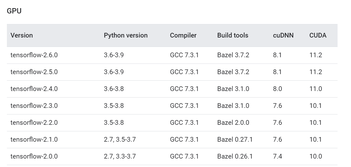
The first, very important step is to go to this link and decide which TF version you want to install. Based on this, the CUDA driver versions and other software versions change.
As of writing this guide, TF 2.6.0 is the latest, and we will be installing that one.
We are only interested in the TF version, cuDNN, and CUDA versions. We keep this tab open and move on to the next step.
Step 2: Install Microsoft Visual Studio
Next, we install Microsoft Visual Studio. Note that this one is different than Visual Studio Code, which is a lightweight IDE so many people love.
Run the downloaded executable and it will take a minute to download the requirements. Then, it will ask you to choose what workloads to install. We don’t want any, so just click install without workloads and click continue. After the installation is done, it will ask you to sign in but you don’t have to.
Step 3: Install the NVIDIA CUDA toolkit
NVIDIA CUDA toolkit contains the drivers for your NVIDIA GPU. Depending on your Windows, they may or may not be already installed. If installed, we should check their version and see if they are compatible with the TensorFlow version we want to install.
Go to your Settings on Windows and choose “Apps & Features”. Then, search for NVIDIA:
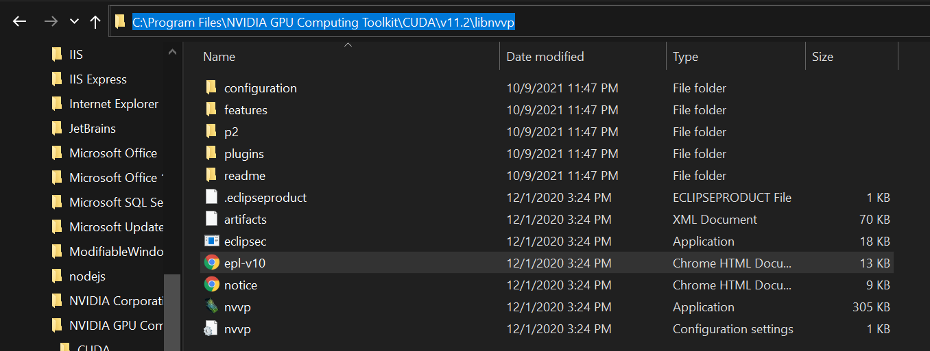
We want to install TF 2.6.0 which requires NVIDIA CUDA Toolkit version 11.2 (see the first link to double-check). If your drivers are any other version, delete all the ones that have “NVIDIA CUDA” in their title (leave the others). Then, go to Local Disk (C:) > Program Files > NVIDIA GPU Computing Toolkit > CUDA. There, you will see a folder with the CUDA version as a name. Delete that folder.
If you search for NVIDIA and no CUDA toolkit is found, go to this page. Here is what it looks like:
Here, we see three 11.2 versions, which are what we need (we got the version from the first TF version link I provided). Click on any of them and choose Windows 10, and download the network installer:
Follow the on-screen prompts and install the drivers with default parameters. Then, restart your computer and come back.
Step 4: Install cuDNN
For TensorFlow 2.6.0, cuDNN 8.1 is required. Go to this page and press download:
It will ask you for an NVIDIA Developer account:
If you don’t have an account already, click “Join now” and enter your email. Fill up the form — the standard stuff. Then, go back to the cuDNN download page:
At the top, it will ask you to fill out a survey. Fill it out and you will be presented with the above page. Click on the first one since it is the one compatible with CUDA Toolkit v. 11.*. There, you will see a Windows version, which you should download.
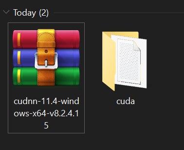
Step 5: Extract the ZIP folder and copy core directories
Extract the downloaded ZIP folder:
Open the cuda folder and copy the three folders at the top (bin, include, lib). Then, go to C:\Program Files\NVIDIA GPU Computing Toolkit\CUDA\v11.2 and paste them there.
Explorer tells you that these folders already exist, which you should press Replace the files in the destination. That’s it, we are done with the software requirements! Restart your computer once again.
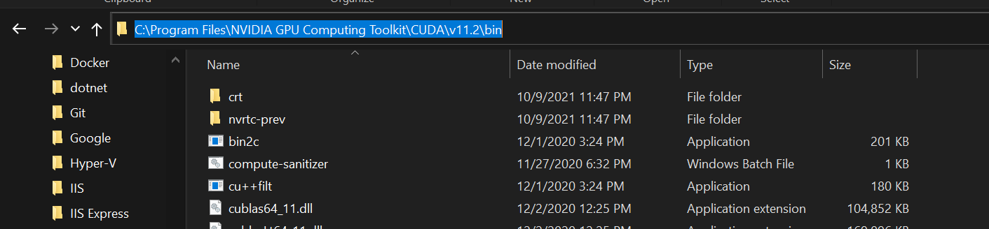
Step 6: Add CUDA toolkit to PATH
Now, it is time to add a few folders to the environment variables. In the last destination, C:\Program Files\NVIDIA GPU Computing Toolkit\CUDA\v11.2, there is a bin and folder:
Open it and copy the file path. Then, press the “Start” (Windows) button and type “Environment variables”:
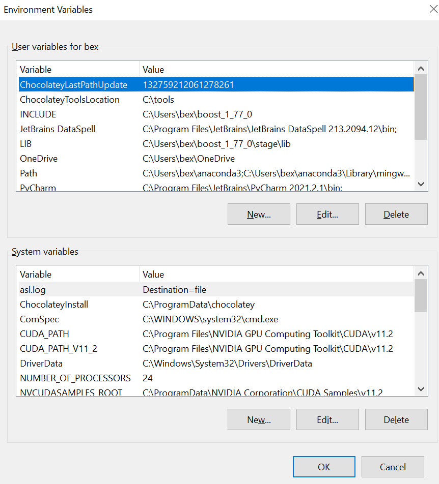
Open it and go to “Environment variables”. This will open this pop-up window:
Choose the “Path” from the top and press edit. Press “New” and paste the copied link there.
Then, go back to the GPU toolkit folder and open the libnvvp folder:
Copy its path and paste it to Environment variables just like you did with the bin folder. Then, close all pop-ups, saving the changes.
Step 7: Install TensorFlow inside a virtual environment with Jupyter Lab
Finally, we are ready to install TensorFlow. Create a virtual environment with your preferred package manager. I use conda, so I create a conda environment named tf with Python version 3.8.
It is important that both TensorFlow and JupyterLab are installed with either pip or conda. You will get a ModelNotFoundError in JupyterLab if they are installed from different channels.
Next, we should add the conda environment to Jupyterlab so that it is listed as a valid kernel when we launch a session:
ipython kernel install --user --name=<name of the kernel, `tf` for our case>
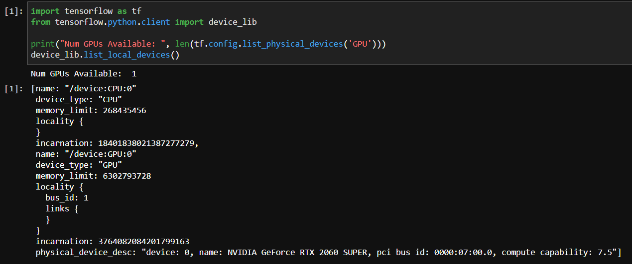
If you launch JupyterLab, you should be able to see the environment as a kernel. Create a new notebook and run this snippet to check if TF can detect your GPU:
import tensorflow as tf from tensorflow.python.client import device_lib
ZeroCostDL4Mic is a toolbox for the training and implementation of common Deep Learning approaches to microscopy imaging. It exploits the ease-of-use and access to GPU provided by Google Colab.
This article describes the techniques and training a deep learning model for image improvement, image restoration, inpainting and super resolution. This utilises many techniques taught in the Fastai course and makes use of the Fastai software library. This method of training a model is based upon methods and research by very talented AI researchers, I’ve credited them where I have been able to in the information and techniques.
As far as I’m aware some of the techniques I’ve applied with the training data are unique at this point with these learning methods (as of February 2019) and only a handful of researchers are using all these techniques together, who will mostly are likely to be Fastai researchers/students.
Super resolution
Super resolution is the process of upscaling and or improving the details within an image. Often a low resolution image is taken as an input and the same image is upscaled to a higher resolution, which is the output. The details in the high resolution output are filled in where the details are essentially unknown.
Super resolution is essentially what you see in films and series like CSI where someone zooms into an image and it improves in quality and the details just appear.
I first heard about ‘AI Super resolution’ last year in early 2018 in the excellent YouTube 2 minute papers, which features short fantastic reviews of the latest AI papers (often longer than 2 minutes). At the time it seemed like magic and I couldn’t understand how it was possible. Definitely living up to the Arthur C Clarke quote “any advanced technology is indistinguishable from magic”. Little did I think that less than a year on I would be training my own super resolution model and writing about it.
This is part of a series of articles I am writing as part of my ongoing learning and research in Artificial Intelligence and Machine Learning. I’m a software engineer and analyst for my day job aspiring to be an AI researcher and Data Scientist.
I’ve written this in part to reinforce my own knowledge and understanding, hopefully this will also be of help and interest to others. I’ve tried to keep the majority of this in as much plain English as possible so that hopefully it will make sense to anyone with a familiarity in machine learning with a some more in depth technical details and links to associates research. These topics and techniques have been quite challenging to understand and its taken me many months to experiment and write this. If you don’t agree with what I’ve written or think it’s just wrong, please do contact me as it’s a continual learning process and I would appreciate feedback.
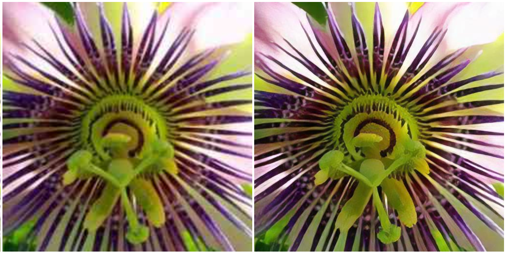
Below is an example of a low resolution image with super resolution performed upon it to improve it:
Left low resolution image. Right super resolution of low resolution image using the model trained here.
The problem deep machine learning based super resolution is trying to solve is that traditional algorithm based upscaling methods lack fine detail and cannot remove defects and compression artifacts. For humans who carry out these tasks manually it is a very slow and painstaking process.
The benefits are gaining a higher quality image from one where that never existed or has been lost, this could be beneficial in many areas or even life saving on medical applications.
Another use case is for compression in transfer between computer networks. Imagine if you only had to send a 256×256 pixel image where a 1024×1024 pixel image is needed.
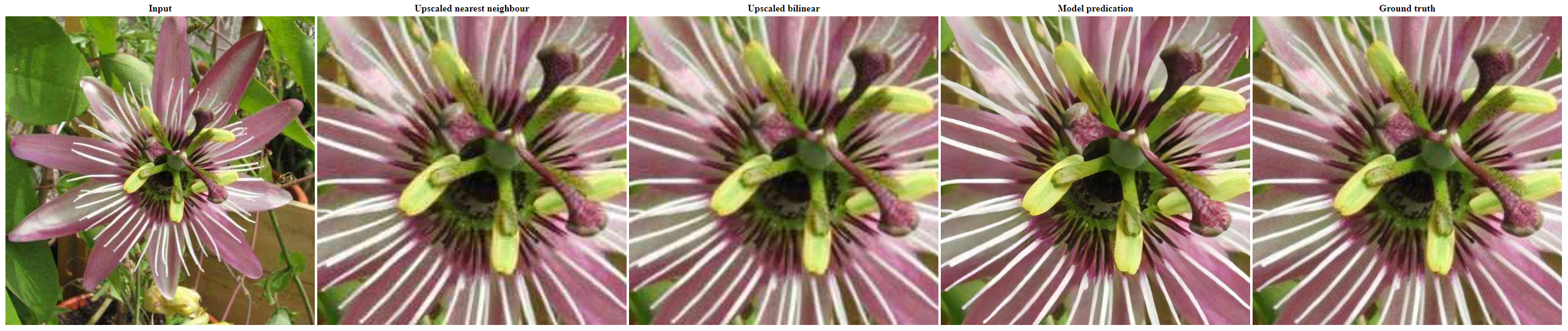
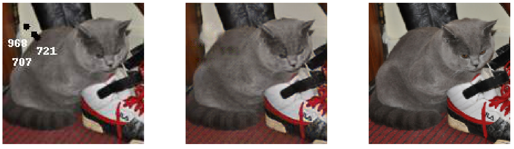
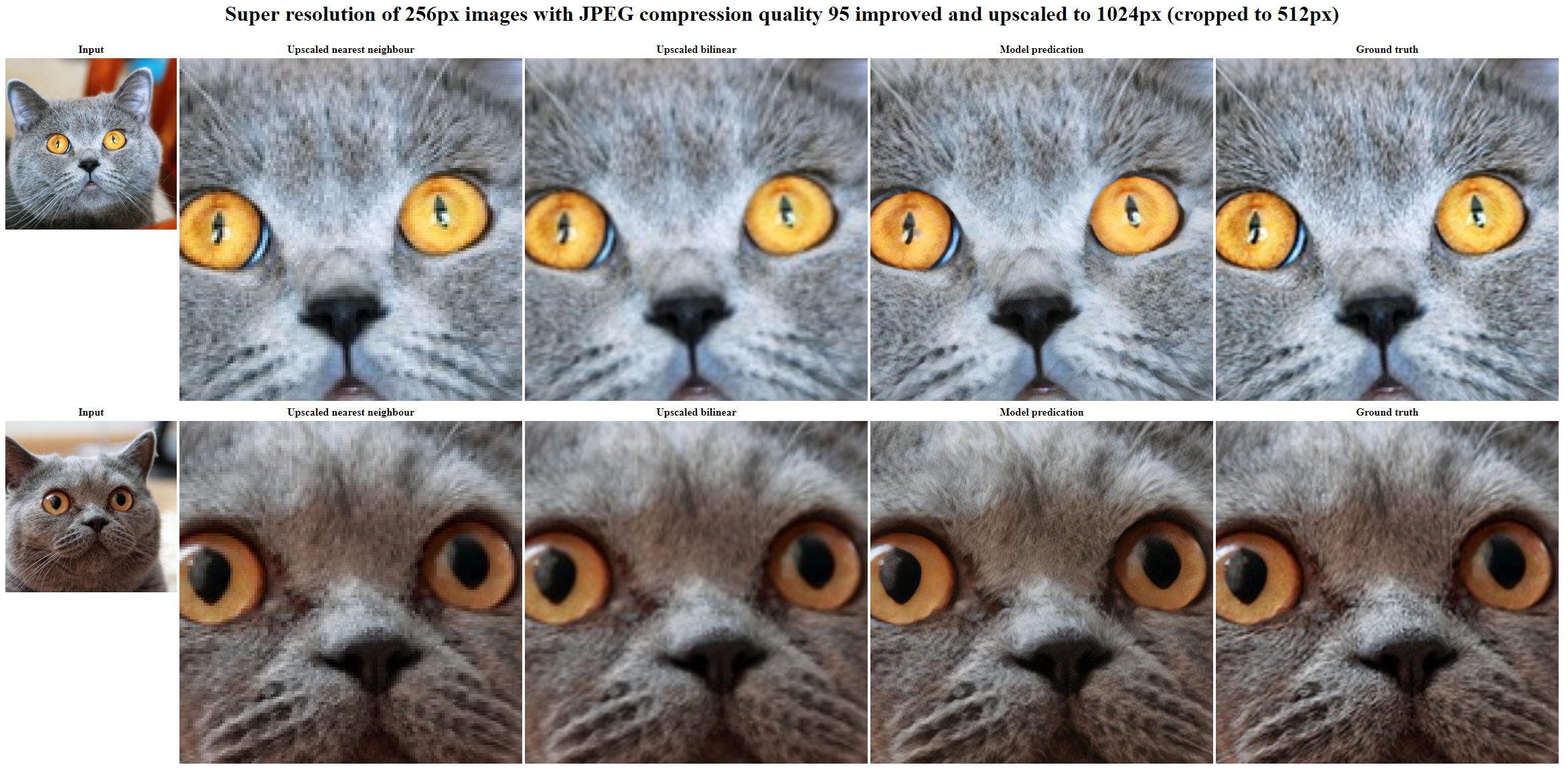
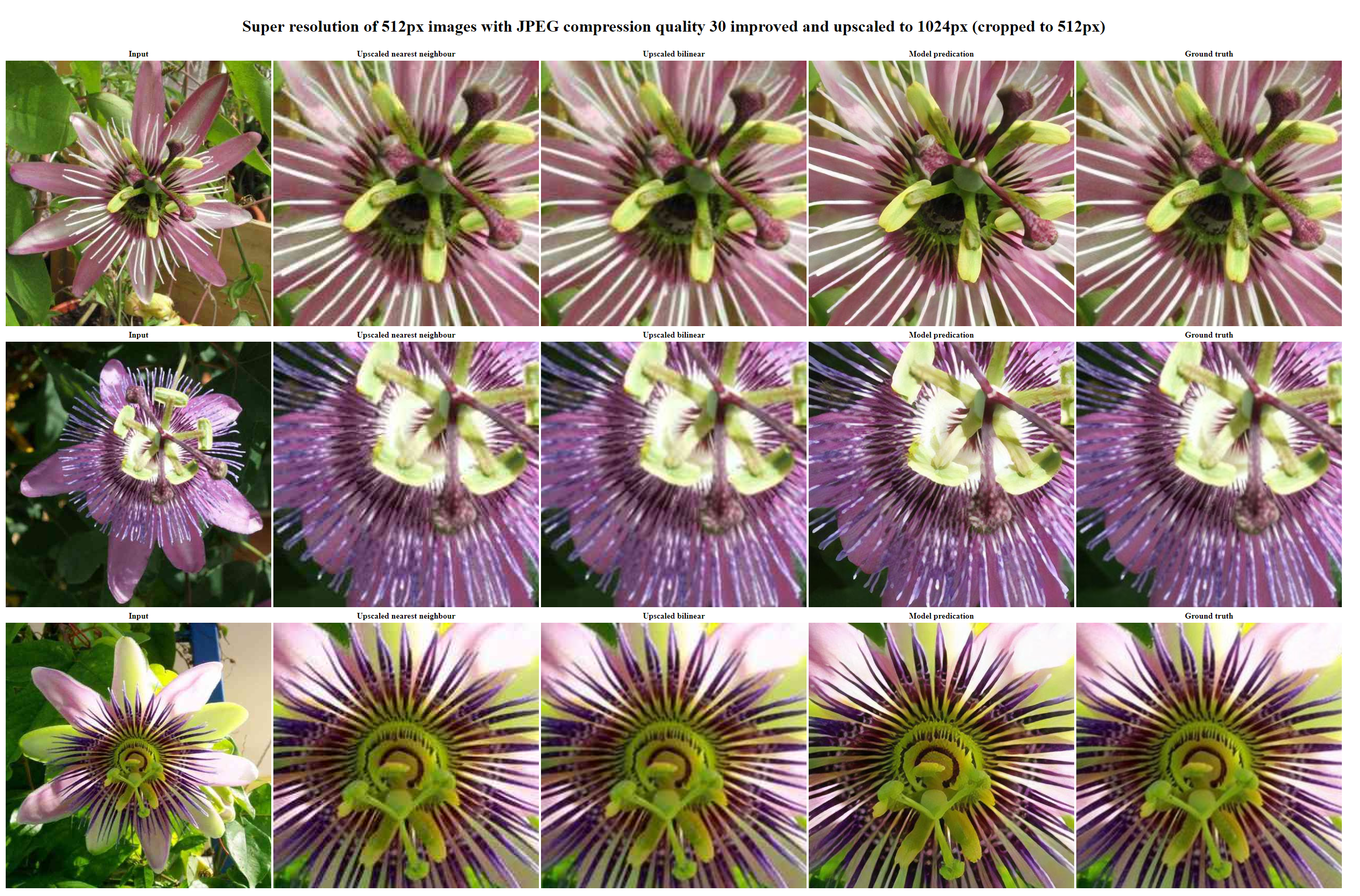
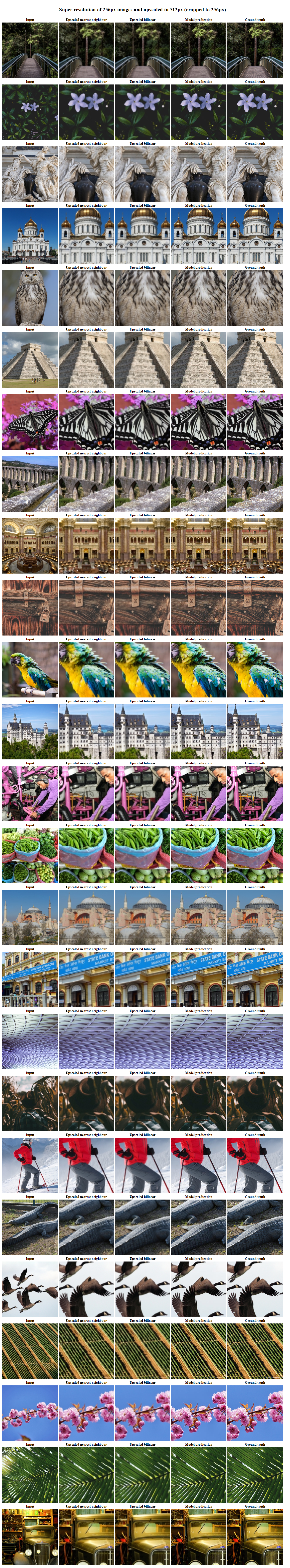
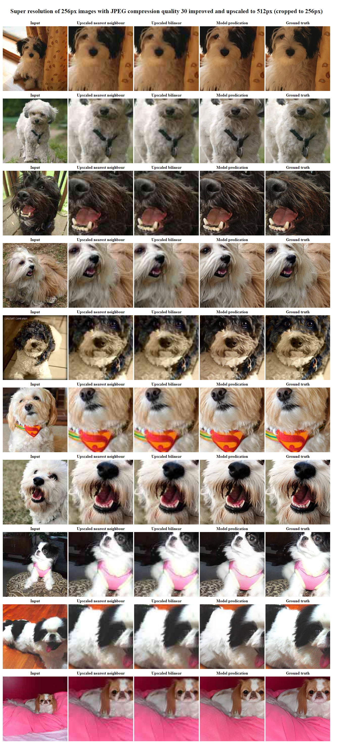
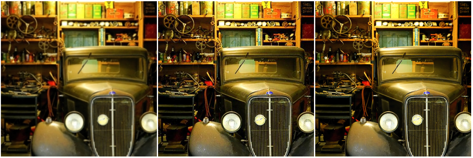
In the set of images below there are five images:
The lower resolution input image to be upscaled
The input image upscaled by nearest neighbour interpolation
The input image upscaled by bi-linear interpretation, this is what your Internet browser would typically need
The input image upscaled and improved by this model’s prediction
The target image or ground truth, which was downscaled to create the lower resolution input.
The objective is to improve the low resolution image to be as good (or better) than than the target, known as the ground truth, which in this situation is the original image we downscaled into the low resolution image.
Comparing the low resolution image, with conventional upscaling, a deep learning model prediction and the target/ground truth
To accomplish this a mathematical function takes the low resolution image that lacks details and hallucinates the details and features onto it. In doing so the function finds detail potentially never recorded by the original camera.
This mathematical function is known as the model and the upscaled image is the model’s prediction.
There are potential ethical concerns with this mentioned at the end of this article, once how the model and its training is explained.
Image repair and inpainting
Models that are trained for super resolution should also be useful for repairing defects in a image (jpeg compression, tears, folds and other damage) as the model has a concept of what certain features should look like, for example materials, fur or even an eye.
Image inpainting is the process of retouching an image to remove unwanted elements in the image, such as a wire fence. For training it is common to cut out sections of the image and train the model to replace the missing parts based on prior knowledge of what should be there. Image inpainting is a usually a very slow process when carried out manually by a skilled human.
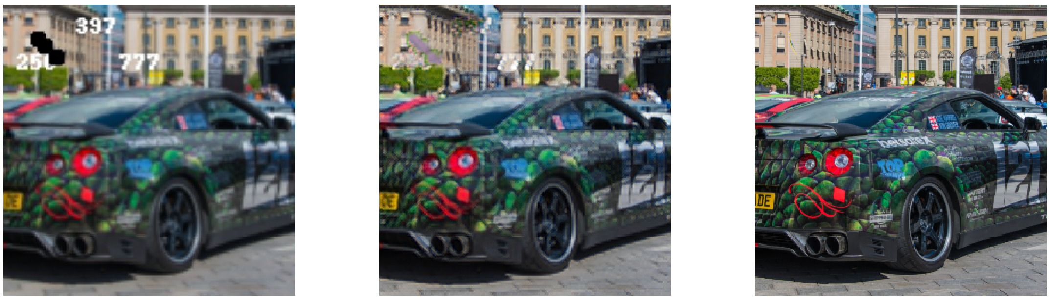
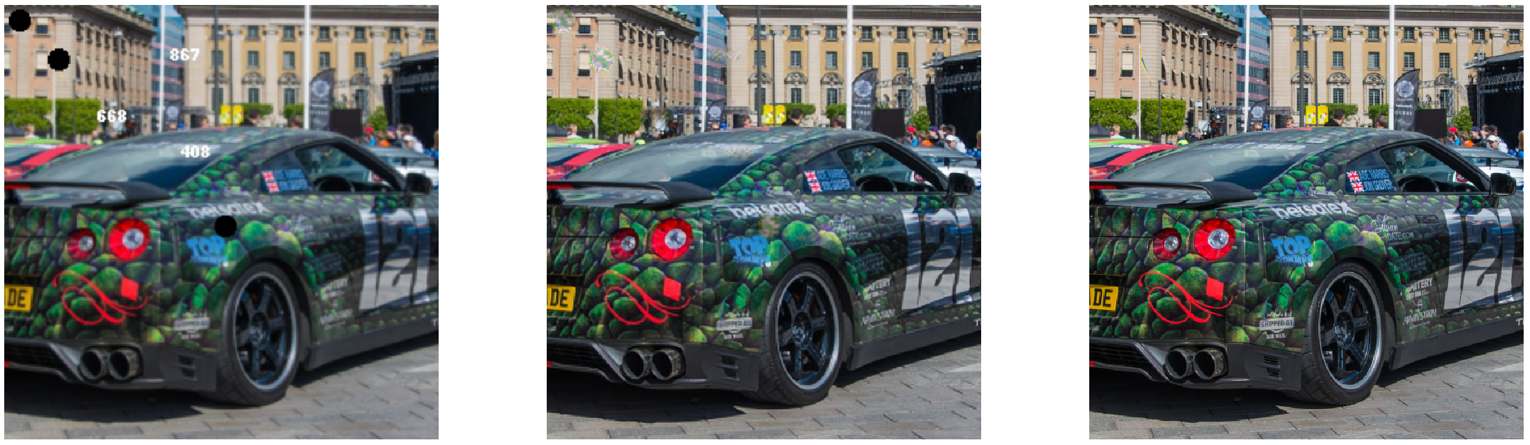
Left an image with holes punched into it and text overlayed. Middle deep learning based model prediction of repaired image. Right the target or Ground truth without defects.
Super resolution and inpainting seem to be often regarded as separate and different tasks. However if a mathematical function can be trained to create additional detail that’s not in an image, then it should be capable of repairing defects and gaps in the the image as well. This assumes those defects and gaps exist in the training data for their restoration to be learnt by the model.
GANs for Super resolution
Most deep learning based super resolution model are trained using Generative Adversarial Networks (GANs).
One of the limitations of GANs is that they are effectively a lazy approach as their loss function, the critic, is trained as part of the process and not specifically engineered for this purpose. This could be one of the reasons many models are only good at super resolution and not image repair.
Universal application
Many deep learning super resolution methods can’t be applied universally to all types of image and almost all have their weaknesses. For example a model trained for the super resolution of animals may not be good for the super resolution of human faces.
The model trained with the methods detailed in this article seemed to perform well across varied dataset including human features, indicating a universal model that is effective at upscaling on any category of image may be possible.
Examples of X2 super resolution
Following are ten examples of X2 super resolution (doubling the image size) from the same model trained on the Div2K dataset, 800 high resolution images of a variety of subject matter categories.
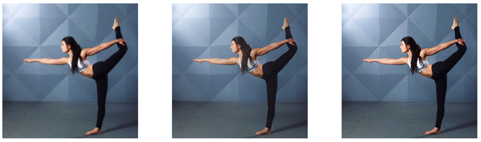
Example one from a model trained on varied categories of image. During early training I had found improving images with humans in had the least improvements and had taken on an more artistic smoothing effect. However this version of the model trained on a generic category data set has managed to improve this image well, look closely at the added detail in the face, the hair, the folds of the clothes and all of the background.
Super resolution on an image from the Div2K validation dataset, example 1
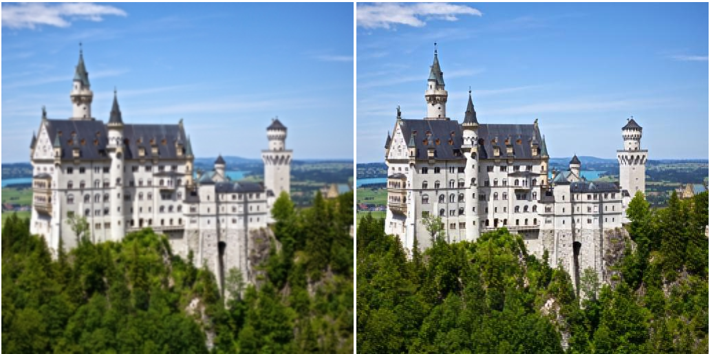
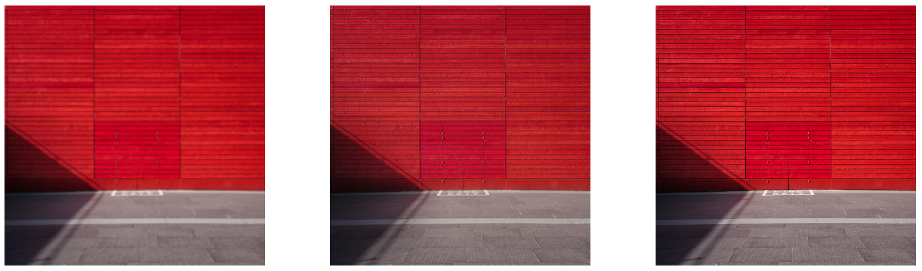
Example two from a model trained on varied categories of image. The model has added detail to the trees, the roof and the building windows. Again impressive results.
Super resolution on an image from the Div2K validation dataset, example 2
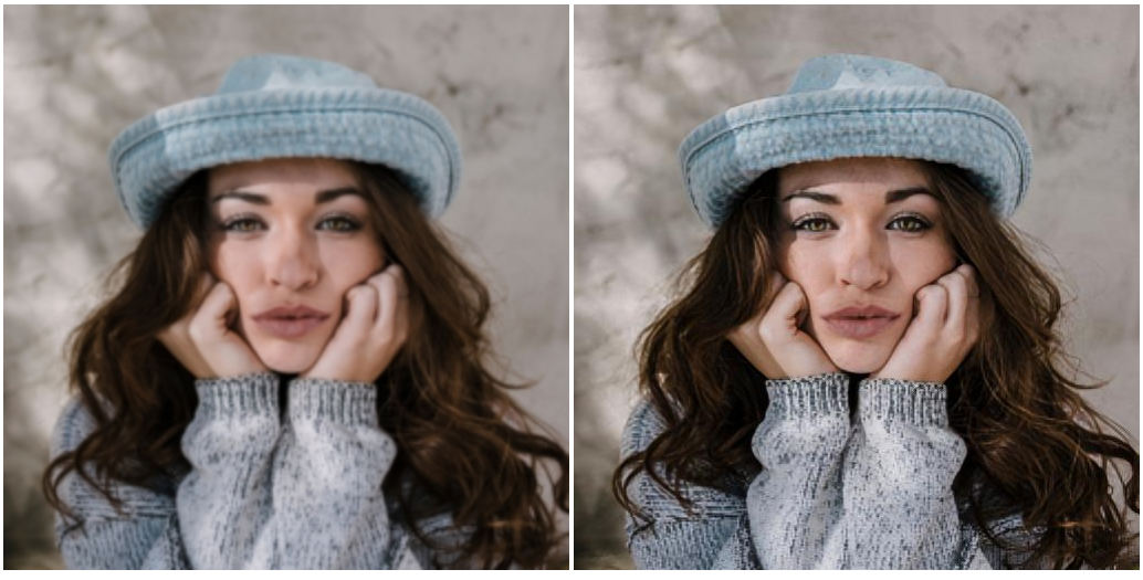
Example three from a model trained on varied categories of image. During training models on different datasets, I had found human faces to had the least pleasing results, however the model here trained on varied categories of images has managed to improve the details in the face and look at the detail added to the hair, this is very impressive.
Super resolution on an image from the Div2K validation dataset, example 3
Example four from a model trained on varied categories of image. The detail added to the pick-axes, the ice, the folds in the jacket and the helmet are impressive here:
Super resolution on an image from the Div2K validation dataset, example 4
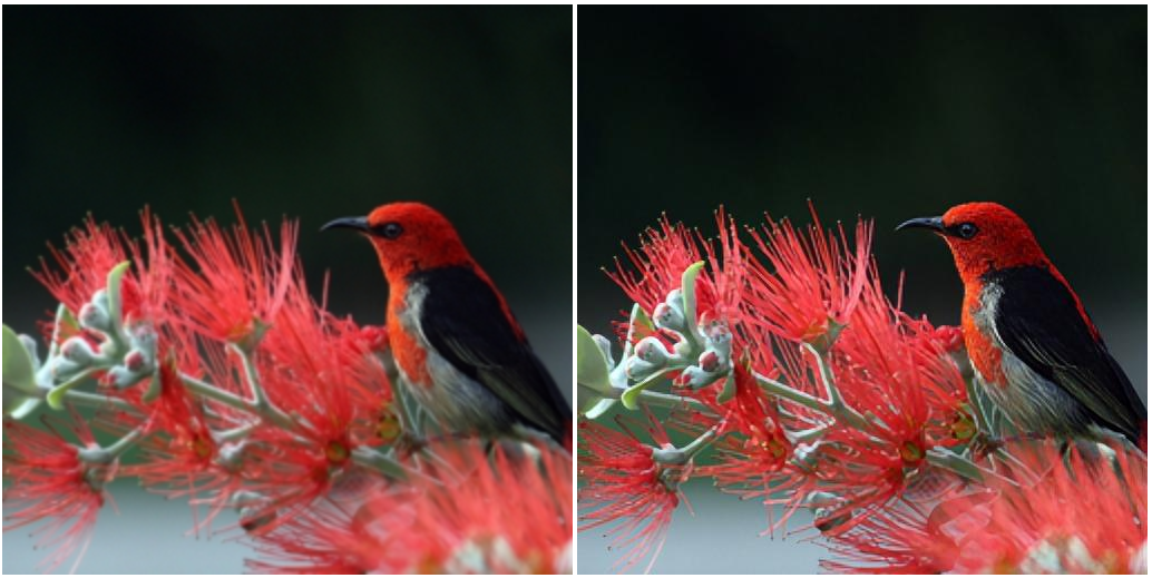
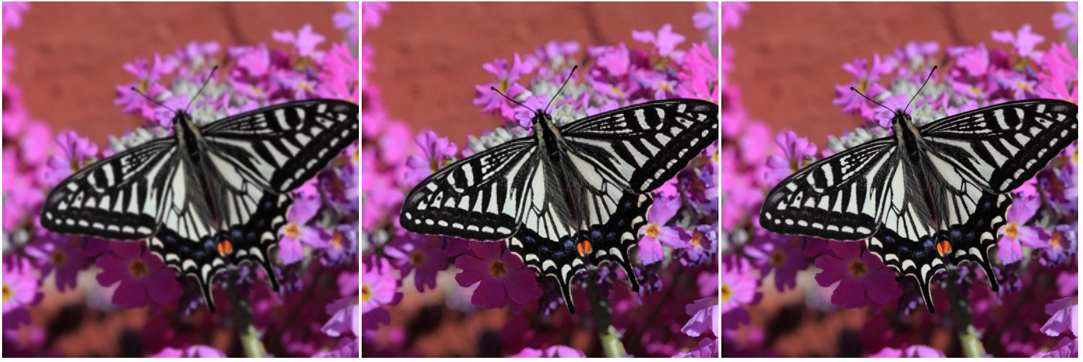
Example five from a model trained on varied categories of image. The improvement of the flowers is really impressive here and the detail on the bird’s eye, beak, fur and wings:
Super resolution on an image from the Div2K validation dataset, example 5
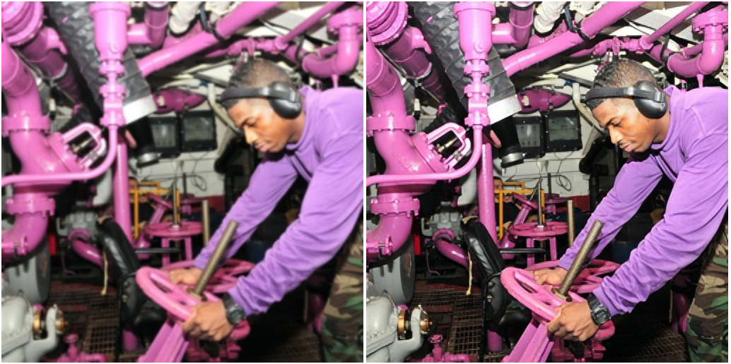
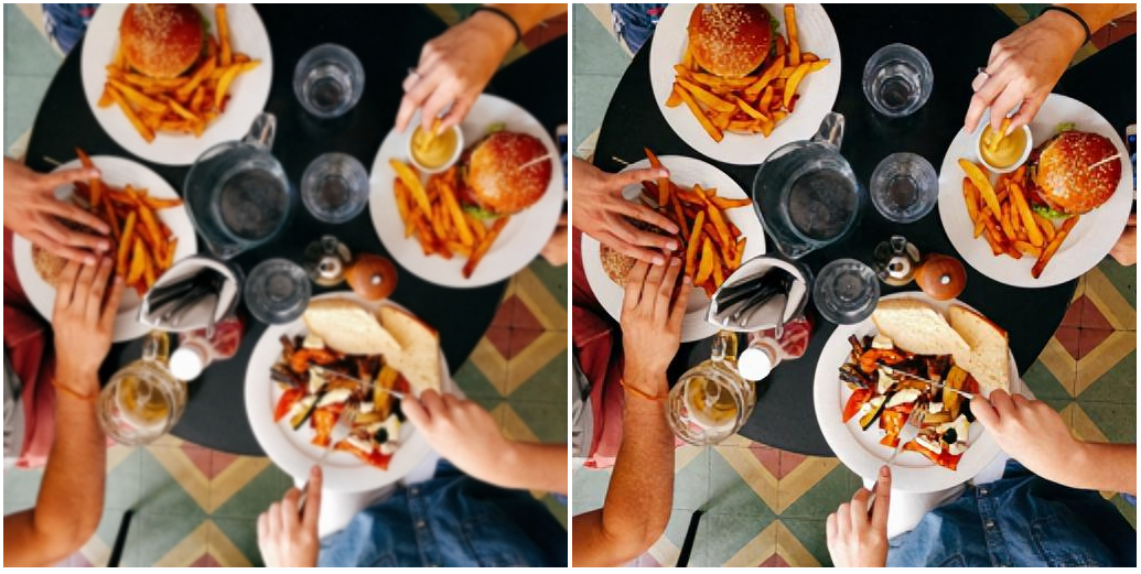
Example six from a model trained on varied categories of image. The model has managed to add detail to the people’s hands, the food, the floor and all the objects. This is really impressive:
Super resolution on an image from the Div2K validation dataset, example 6
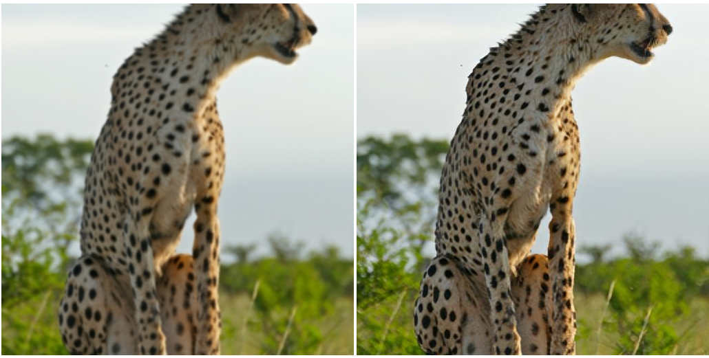
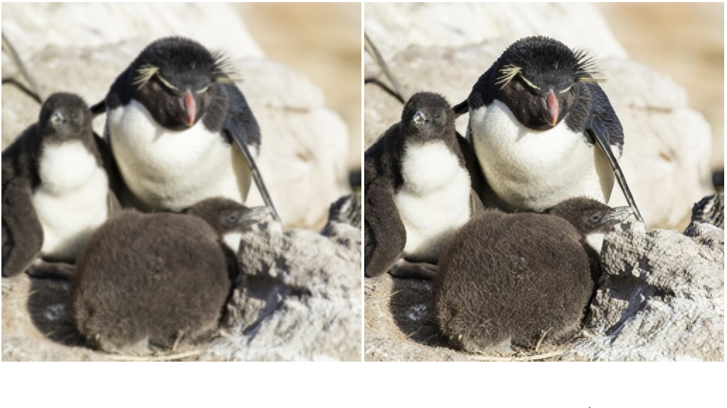
Example seven from a model trained on varied categories of image. The model has brought the fur into focus and kept the background blurred:
Super resolution on an image from the Div2K validation dataset, example 7
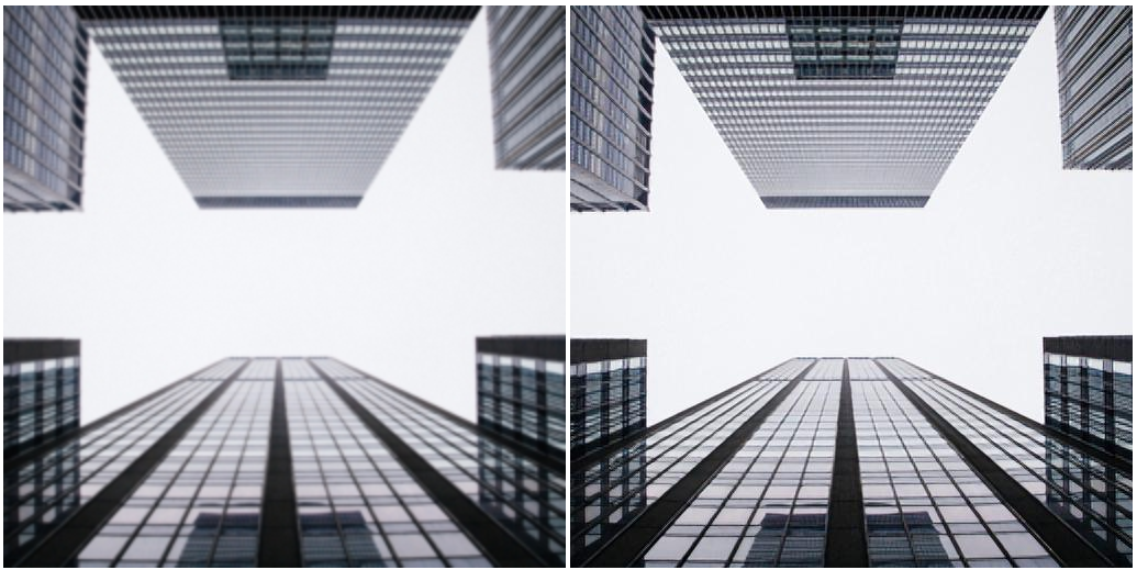
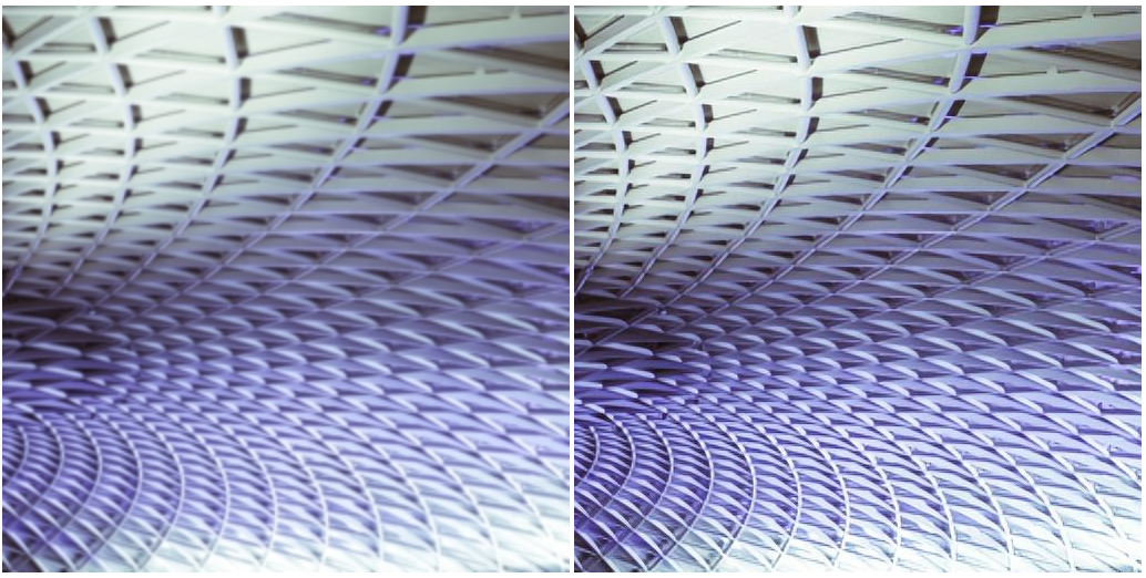
Example eight from a model trained on varied categories of image. The model has done well to sharpen up the lines between the windows:
Super resolution on an image from the Div2K validation dataset, example 8
Example nine from a model trained on varied categories of image. The detail of the fur really seems to have been imagined by the model.
Super resolution on an image from the Div2K validation dataset, example 9
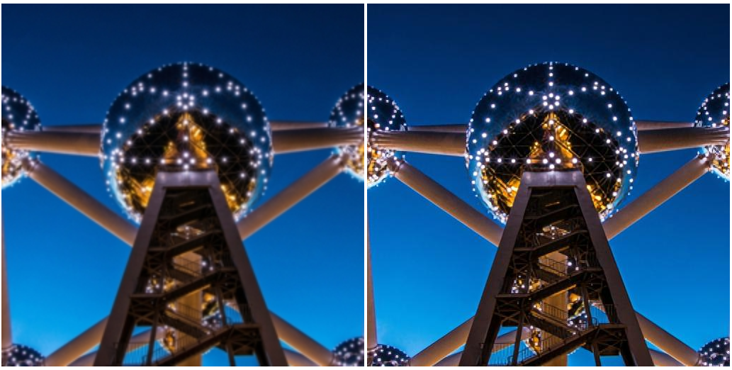
Example ten from a model trained on varied categories of image. This really seems impressive sharpening around the lines of the structure and the lights.
Super resolution on an image from the Div2K validation dataset, example 10.
Example eleven from a model trained on varied categories of image. The improvement and sharpening of the feathers is very noticeable.
Super resolution on an image from the Div2K validation dataset, example 11.
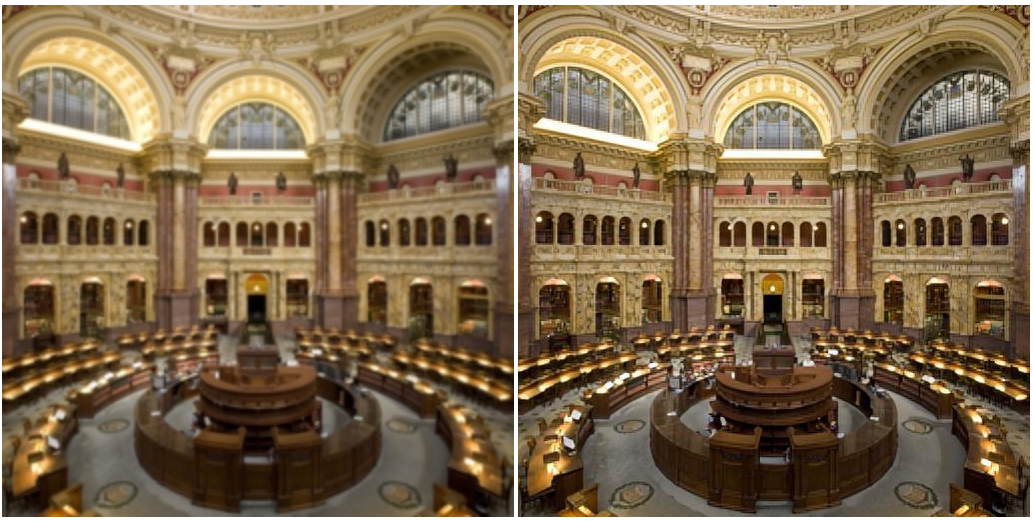
Example twelve from a model trained on varied categories of image. This interior images has been subtly improved almost everywhere.
Super resolution on an image from the Div2K validation dataset, example 12.
Example thirteen from a model trained on varied categories of image. This is the last example in this section, a complex image that’s been sharpened and improved.
Super resolution on an image from the Div2K validation dataset, example 13.
This model’s predictions having performed super resolution
All the images above were improvements made on validation image sets during or at the end of training.
The trained model has been used to create upscaled images of over 1 megapixel, these are a few of the best examples:
In this first example a 256 pixel square image saved at high JPEG quality (95) is inputted into the model that upscales the image to a 1024 pixel square image performing X4 super resolution:
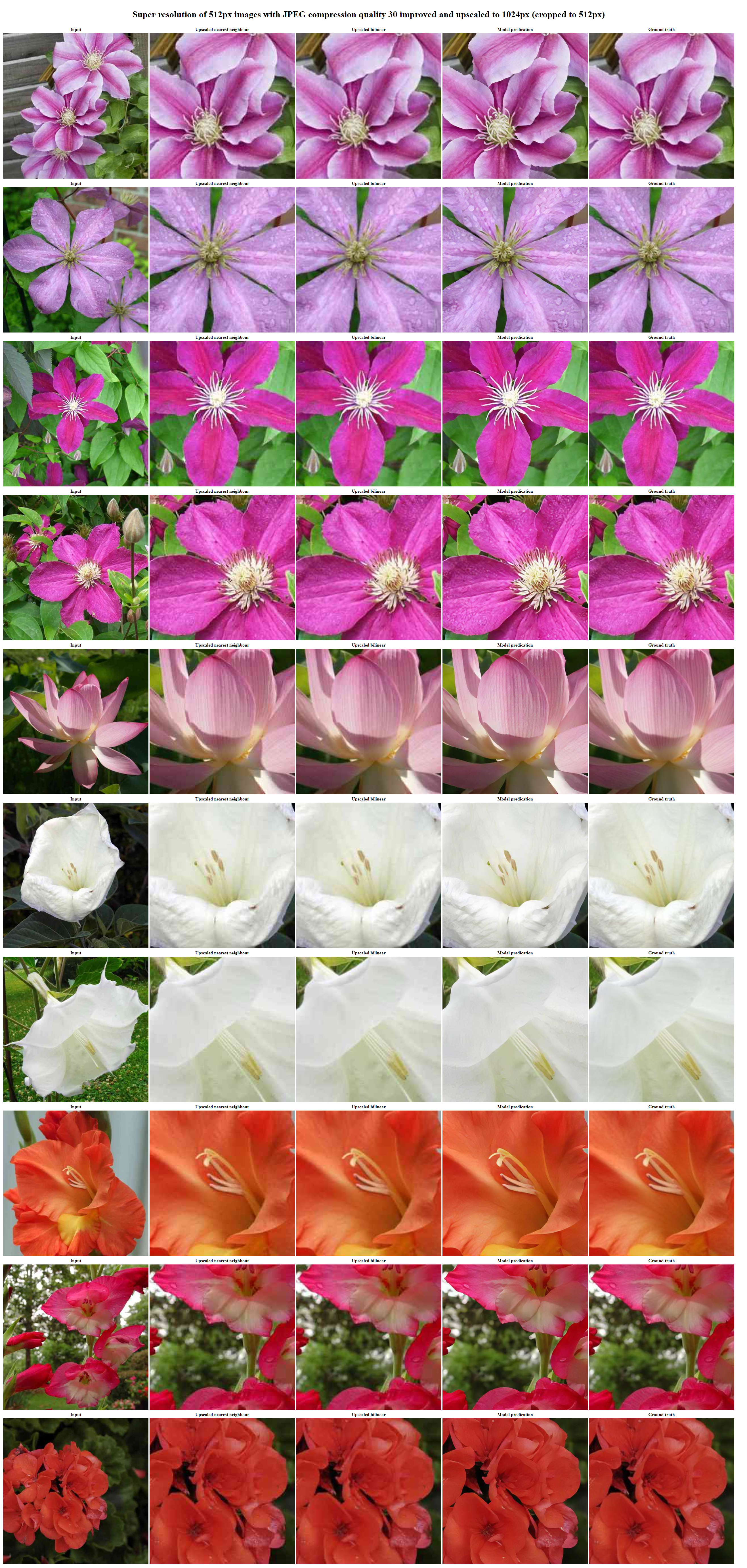
In the next example a 512 pixel image saved at low JPEG quality (30) is inputted into the model that upscales the image to a 1024 pixel square image performing X2 super resolution on a lower quality source image. Here the model’s prediction I believe looks better than the target ground truth image, which is amazing:
Passes it through a trained mathematical function which is a type of neural network
Outputs an image of the same size or larger that is an improvement over the input.
This builds on the techniques suggested in the Fastai course by Jeremy Howard and Rachel Thomas. It uses the Fastai software library, the PyTorch deep learning platform and the CUDA parallel computation API.
The Fastai software library breaks down a lot of barriers to getting started with complex deep learning. As it is open source it’s easy to customise and replace elements of your architecture to suit your prediction tasks, if needed. This image generator model is build on top of the Fastai U-Net learner.
This method uses the following, each of which is explained further below:
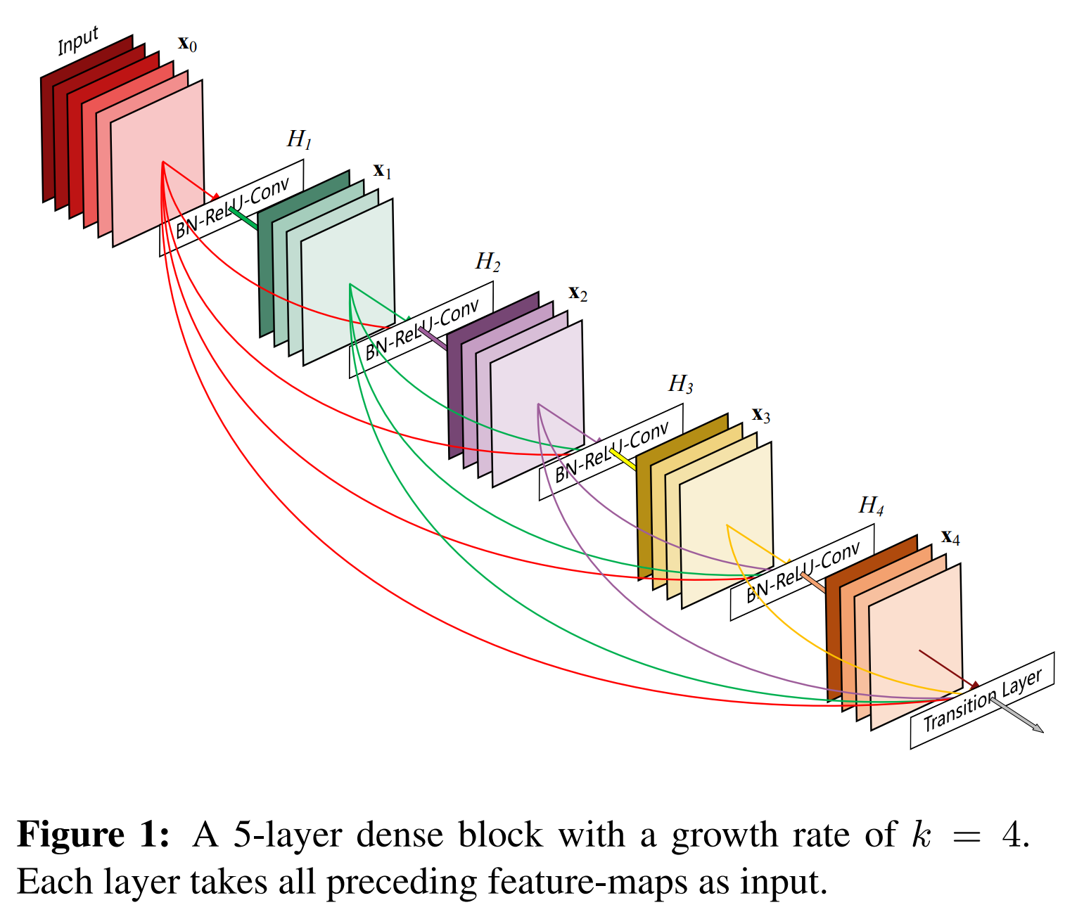
A U-Net architecture with cross connections similar to a DenseNet
A ResNet-34 based encoder and a decoder based on ResNet-34
Pixel Shuffle upscaling with ICNR initialisation
Transfer learning from pretrained ImageNet models
A loss function based on activations from a VGG-16 model, pixel loss and gram matrix loss
Discriminative learning rates
Progressive resizing
This model or mathematical function has over 40 million parameters or coefficients allowing it to attempt to preform super resolution.
Residual Networks (ResNet)
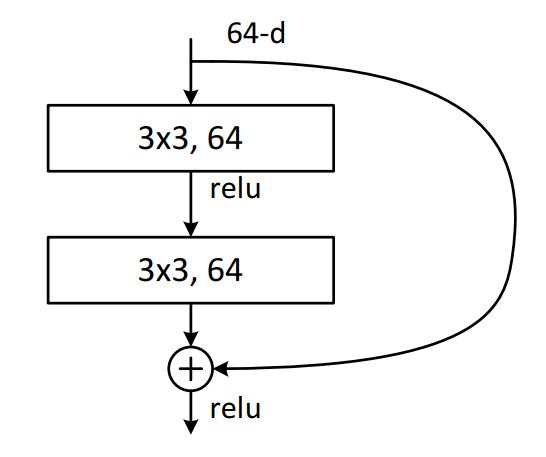
ResNet is a Convolutional Neural Network (CNN) architecture, made up of series of residual blocks (ResBlocks) described below with skip connections differentiating ResNets from other CNNs.
When first devised ResNet won that year’s ImageNet competition by a significant margin as it addressed the vanishing gradient problem, where as more layers are added training slows and accuracy doesn’t improve or even gets worse. It is the networks skip connections that accomplish this feat.
These are shown in the diagram below and explained in more detail as each ResBlock within the ResNet is described.
Left 34 Layer CNN, right 34 Layer ResNet CNN. Source Deep Residual Learning for Image Recognition: https://arxiv.org/abs/1512.03385
Residual blocks ( ResBlocks) and dense blocks
Convolutional networks can be substantially deeper, more accurate, and more efficient to train if they contain shorter connections between layers close to the input and those close to the output.
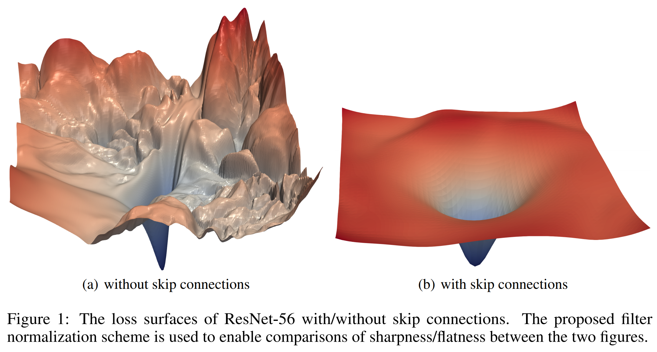
If you visualise the loss surface (the search space for the varying loss of the model’s prediction), this looks like a series of hills and valleys as the left hand image in the diagram below shows. The lowest loss is the lowest point. Research has shown that a smaller optimal network can be ignored even if it’s an exact part of a bigger network. This is because the loss surface is too hard to navigate. This means that by adding layers to the model it can make the prediction become worse.
Loss surface with and without skip connections. Source: Visualising loss space in Neural networks: https://arxiv.org/abs/1712.09913
A solution that’s been very effective is to add cross connections between layers of the network allowing large sections to be skipped if needed. This creates a loss surface that looks like the image on the right. This is much easier for the model to be trained with optimal weights to reduce the loss.
Each ResBlock has two connections from its input, one going through a series of convolutions, batch normalisation and linear functions and the other connection skipping over that series of convolutions and functions. These are known as an identity, cross or skip connections. The tensor outputs of both connections are added together.
Densely Connected Convolutional Networks and DenseBlocks
Where a ResBlock provides an output that is a tensor addition, this can be changed to be tensor concatenation. With each cross/skip connection the network becomes more dense. The ResBlock then becomes a DenseBlock and the network becomes a DenseNet.
This allows the computation to skip over larger and larger parts of the architecture.
Due to the concatenation DenseBlocks consume a lot of memory compared to other architectures and are very well suited to smaller datasets.
U-Nets
A U-Net is a convolutional neural network architecture that was developed for biomedical image segmentation. U-Nets have been found to be very effective for tasks where the output is of similar size as the input and the output needs that amount of spatial resolution. This makes them very good for creating segmentation masks and for image processing/generation such as super resolution.
When convolutional neural nets are commonly used with images for classification, the image is taken and downsampled into one or more classifications using a series of stride two convolutions reducing the grid size each time.
To be able to output a generated image of the same size as the input, or larger, there needs to be an upsampling path to increase the grid size. This makes the network layout resemble a U shape, a U-Net the downsampling/encoder path forms the left hand side of the U and the upsampling/decoder path forms the right hand part of the U.
For the upsampling/decoder path several transposed convolutions accomplishes this, each adding pixels between and around the existing pixels. Essentially the reverse of the downsampling path is carried out. The options for the upsampling algorithms are discussed further on.
Note that this model’s U-Net based architecture also has cross connections which are detailed further on, these weren’t part of the original U-Net architecture.
Each upsample in the decoder/upsampling part of the network (right hand part of the U) needs to add pixels around the existing pixels and also in-between the existing pixels to eventually reach the desired resolution.
This process can be visualised as below from the paper “A guide to convolution arithmetic for deep learning” where zeros are added between the pixels. The blue pixels are the original 2×2 pixels being expanded to 5×5 pixels. 2 pixels of padding around the outside are added and also a pixel between each pixel. In this example all new pixels are zeros (white).
Adding pixels around and between the pixels. Source: A guide to convolution arithmetic for deep learning: https://arxiv.org/abs/1603.07285
This could have been improved with some simple initialisation of the new pixels by using the weighted average of the pixels (using bi-linear interpolation), as otherwise it is unnecessarily making it harder for the model to learn.
In this models it instead uses an improved method known as pixel shuffle or sub-pixel convolution with ICNR initialisation, which results in the gaps between the pixels being filled much more effectively. This is described in the paper “Real-Time Single Image and Video Super-Resolution Using an Efficient Sub-Pixel Convolutional Neural Network”.
Pixel shuffle. Source: Real-Time Single Image and Video Super-Resolution Using an Efficient Sub-Pixel Convolutional Neural Network, source: https://arxiv.org/abs/1609.05158
The pixel shuffle upscales by a factor of 2, doubling the dimensions in each of the channels of the image (in its current representation at that part of the network). Replication padding is then performed to provide an extra pixel around the image. Then average pooling is performed to extract features smoothly and avoid the checkerboard pattern which results from many super resolution techniques.
After the representation for these new pixels are added, the subsequent convolutions improve the detail within them as the path continues through the decoder path of the network before then upscaling another step and doubling the dimensions.
U-Nets and fine image detail
When using a only a U-Net architecture the predictions tend to lack fine detail, to help address this cross or skip connections can be added between blocks of the network.
Rather than adding a skip connection every two convolutions as is in a ResBlock, the skip connections cross from same sized part in downsampling path to the upsampling path. These are the grey lines shown in the diagram above.
The original pixels are concatenated with the final ResBlock with a skip connection to allow final computation to take place with awareness of the original pixels inputted into the model. This results in all of the fine details of the input image are at the top on the U-Net with the input mapped almost directly to the output.
The outputs of the U-Net blocks are concatenated making them more similar to DenseBlocks than ResBlocks. However there are stride two convolutions that reduce the grid size back down, which also helps to keep memory usage from growing too large.
ResNet-34 Encoder
ResNet-34 is a 34 layer ResNet architecture, this is used as the encoder in the downsampling section of the U-Net (the left half of the U).
The Fastai U-Net learner when provided with an encoder architecture will automatically construct the decoder side of the U-Net architecture, in the case transforming the ResNet-34 encoder into a U-Net with cross connections.
For an image generation/prediction model to know how to do perform its prediction effectively it vastly speeds up training time if a pretrained model is used. The model then has a starting knowledge of the kind of features that need to be detected and improved. Using a model and weights that have been pre-trained on ImageNet is an excellent start when photographs are used as inputs.. The pretrained ResNet-34 for pyTorch is available from Kaggle: https://www.kaggle.com/pytorch/resnet34
Loss Function
The loss function is based upon the research in the paper Losses for Real-Time Style Transfer and Super-Resolution and the improvements shown in the Fastai course (v3).
This paper focuses on feature losses (called perceptual loss in the paper). The research did not use a U-Net architecture as the machine learning community were not aware of them at that time.
Source: Convolutional Neural Network (CNN) Perceptual Losses for Real-Time Style Transfer and Super-Resolution: https://arxiv.org/abs/1603.08155
This model used here is trained with a similar loss function to the paper, using VGG-16 but also combined with pixel mean squared error loss loss and gram matrix loss. This has been found to be very effective by the Fastai team.
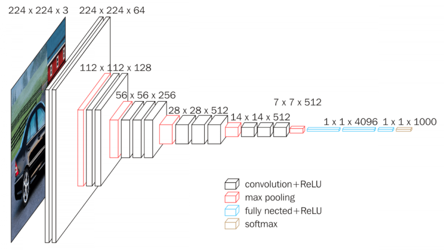
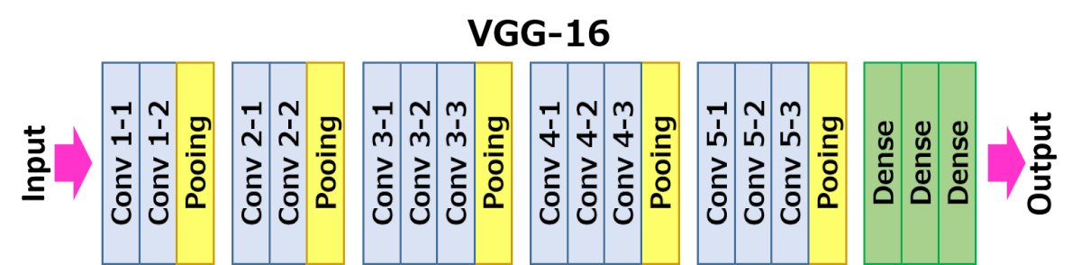
VGG-16
VGG is another CNN architecture devised in 2014, the 16 layer version is utilised in the loss function for training this model.
The VGG model. a network pretrained on ImageNet, is used to evaluate the generator model’s loss. Normally this would be used as a classifier to tell you what the image is, for example is this a person, a dog or cat.
The head of the VGG model is ignored and the loss function uses the intermediate activations in the backbone of the network, which represent the feature detections. The head and backbone of networks are described a little further in the training section further on.
Those activations can be found by looking through the VGG model to find all the max pooling layers. These are where the grid size changes and features are detected.
Heatmaps visualising the activations for varied images can be seen in the image below. This shows examples of varied features detected in the different layers of network.
The training of this super resolution model uses the loss function based on the VGG model’s activations. The loss function remains fixed throughout the training unlike the critic part of a GAN.
The Feature map has 256 channels by 28 by 28 which are used to detect features such fur, an eyeball, wings and the type material among many other type of features. The activations at the same layer for the (target) original image and the generated image are compared using mean squared error or the least absolute error (L1) error for the base loss. These are feature losses. This error function uses L1 error.
This allows the loss function to know what features are in the target ground truth image and to evaluate how well the model’s prediction’s features match these rather than only comparing pixel difference.
Training details
The training process begins with a model as described above: a U-Net based on the ResNet-34 architecture pretrained on ImageNet using a loss function based on the VGG-16 architecture pretrained on ImageNet combined with pixel loss and a gram matrix.
Training data
With super resolution it is fortunate in most applications there is an almost infinite amount of data can be created as a training set. If a set of high resolution images is acquired, these can be encoded/resized to smaller images, so that we have a training set with a low resolution and high resolution image pair. The prediction from our model can then be used evaluated against the high resolution image.
The low resolution image is initially a copy of the target/ground truth image at half the dimensions. The low resolution image is then initially upscaled using bi-linear transformation to make it the same dimensions as the target image to input into the U-Net based model.
The actions taken in this method of creating the training data are what the model learns to fit (reversing the process).
The training data can be further augmented by:
Randomly reducing the quality of the image within bounds
Taking random crops
Flipping the image horizontally
Adjusting the lighting of the image
Adding perspective warping
Randomly adding noise
Randomly punching small holes into the image
Randomly adding overlaid text or symbols
The images below are an example of data augmentation, all of these were generated from the same source image:
Example of data augmentation
Changing the quality reduction and noise to be random for each image improved the resulting model allowing it to learn how to improve all of these different forms of image degradation and to better generalise.
Feature and quality improvement
The U-Net based model enhances the details and features in the upscaled image generating an improved image though the function containing approximately 40 million parameters.
Training the head and the backbone of the model
Three methods used here in particular help the training process. These are progressive resizing, freezing then unfreezing the gradient descent update of the weights in the the backbone and discriminative learning rates.
The model’s architecture is split into two parts, the backbone and the head.
The backbone is the left hand section of the U-Net, the encoder/down-sampling part of the network based on ResNet-34. The head is the right hand section of the U-Net, the decoder/up-sampling part of the network.
The backbone has pretrained weights based on ResNet34 trained on ImageNet, this is the transfer learning.
The head needs its weights training as these layers’ weights are randomly initialised to produce the desired end output.
At the very start the output from the network is essentially random changes of pixels other than the Pixel Shuffle sub-convolutions with ICNR initialisation used as the first step in each upscale in the decoder/upsampling path of the network.
Once trained the head on top of the backbone allows the model to learn to do something different with its pretrained knowledge in the backbone.
Freeze the backbone, train the head
The weights in the backbone of the network are frozen so that only the weights in the head are initially being trained.
A learning rate finder is run for 100 iterations and plots the graph of loss against learning rate, a point around the steepest slope down towards the minimum loss is selected as the maximum learning rate. Alternatively a rate 10 times less than the lowest point can be used to see if that performs any better.
Learning rate against loss, optimal slope with backbone frozen
The fit one cycle policy is used to vary learning rate and momentum, described in detail in Leslie Smith’s paper
It’s faster to train on larger numbers of smaller images initially and then scale up the network and training images. Upscaling and improving an image to 128px by 128px image from 64px by 64px is a much easier task than performing that operation on a larger image and much quicker on a larger dataset. This is called progressive resizing, it also helps the model to generalise better as is sees many more different images and less likely to be overfitting.
The process is to train with small images in larger batches, then once the loss is decreasing to an acceptable level then a new model is created that accepts larger images transferring the learning from the model trained on smaller images.
As the training image size increases the batch size has to decreased to avoid running out of memory, as each batch contains larger images with four times as many pixels in each.
Note that the defects in the input image have been randomly added to improve the restorative properties of the model and to help it generalise better.
Examples from the validation set separated from the training set are shown here at some of the progressive sizes:
At each image size training of one cycle of 10 epochs is carried out. This is with the backbone weights, frozen.
The image size is doubled and the model updated with the additional grid sizes for the path of larger images through the network. It’s important to note the number of weights does not change.
Step 1: upscale from 32 pixels by 32 pixels to 64 pixels by 64 pixels. A learning rate of 1e-2 was used.
Super resolution to 64px by 64px on a 32px by 32px image from the validation set. Left low resolution input, middle super resolution models prediction, right target/ground truth.
Step 2: upscale from 64 pixels by 64 pixels to 128 pixels by 128 pixels. A learning rate of 2e-2 was used.
Super resolution to 128px by 128px on a 64px by 64px image from the validation set. Left low resolution input, middle super resolution models prediction, right target/ground truth
Step 3: upscale from 128 pixels by 128 pixels to 256 pixels by 256 pixels. Discriminative learning rates between 3e-3 and 1e-3 were used.
Super resolution to 256px by 256px on a 128px by 128px image from the validation set. Left low resolution input, middle super resolution models prediction, right target/ground truth
Step 4: upscale from 256 pixels by 256 pixels to 512 pixels by 512 pixels. Discriminative learning rates between 1e-3 and were used.
Super resolution to 512px by 512px on a 256px by 256px image from the validation set. Left low resolution input, middle super resolution models prediction, right target/ground truth
Unfreeze the backbone
The backbone is split into two layer groups and the head is a third layer group.
The weights of the entire model are then unfrozen and the model is trained with discriminative learning rates. These learning rates are much smaller in the first layer group then increased in the second layer group and increased again in the head, the last layer group.
The learning rate finder is run again with the backbone and head unfrozen.
Learning rate against loss with backbone and head unfrozen
Discriminative learning rates between 1e-6 and 1e-4 were used. The learning rate in the head is still an order of magnitude less than in the previous cycle of learning, where only the head was unfrozen. This allows fine-tuning of the model without risking losing much of the accuracy already found. This is known as learning rate annealing, where the learning rate is reduced as we approach the optimal loss.
Continuing training on larger input images would improve the quality of super resolution, however the batch size has to keep shrinking to fit within memory constraints and training time increases and limits of my training infrastructure was reached.
All training was carried out on a Nvidia Tesla K80 GPU with 12GB RAM and in less than 12 hours from start to finish with the progressive resizing.
Results
The above images in the progressive resizing section of training, show how effective deep learning based super resolution is at improving the detail, removing watermarks, defects and impainting missing details.
The next three image predictions based on images form the Div2K dataset all had super resolution performed on them by the same trained model, showing a deep learning super resolution model might be able universally applied.
Note: these are from the actual Div2K training set, although that set was split into my own training and validation datasets and the model did not see these images during training. There are further examples from the actual Div2K validation set further on.
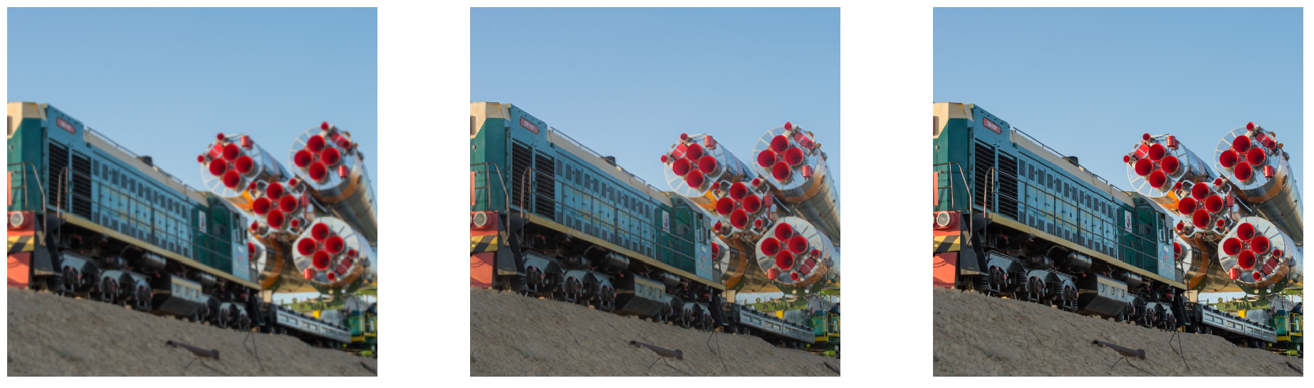
Left: 256 x 256 pixel input. Middle: 512 x 512 prediction from the model. Right: 512 x 512 pixel ground truth target. Looking at the vents on front of the train, the detail improvement is clear and very close to the ground truth target.
256 by 256 pixel super resolution to 512 by 512 pixel image, example 1
Left: 256 x 256 pixel input. Middle: 512 x 512 prediction from the model. Right: 512 x 512 pixel ground truth target. The feature improvement in the image prediction below here is quite amazing. During my early training attempts I had almost concluded super resolution of human features would be a task too complex.
256 by 256 pixel super resolution to 512 by 512 pixel image, example 2
Left: 256 x 256 pixel input. Middle: 512 x 512 prediction from the model. Right: 512 x 512 pixel ground truth target. Notice how the white “Fire Exit” text and the paneling lines have been improved.
256 by 256 pixel super resolution to 512 by 512 pixel image, example 3
Model prediction comparison on the Div2K validation dataset
Super resolution on the Oxford 102 Flowers dataset
The super resolution results from a separate trained model on a dataset of images of flowers I think is quite outstanding, many of the model predictions actually look sharper than the ground truth having truly performed super resolution upon the validation set (images not seen during training).
Validation results upscaling images from the Oxford 102 Flowers dataset consisting of 102 flower categories
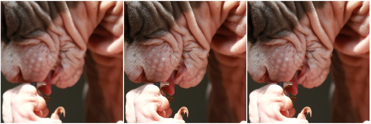
Super resolution on the Oxford-IIIT Pet dataset
The example below from a separate trained model upscaling low resolution images of dogs is very impressive, again from the validation set, creating finer details of fur, sharpening eyes and noses and really improving the features in the images. Most of the upscaled images are close to being as good as the ground truth and certainly much better than the bilinear upscaled images.
Validation results upscaling images from Oxford-IIIT Pet dataset, a 37 category pet dataset with roughly 200 images for each class.
These results I believe are impressive, the model must have developed a ‘knowledge’ of what a group of pixels must have been in the original subject of the photograph/image.
It knows that certain areas are blurred and knows to reconstruct a blurred background.
The model couldn’t do this if it hadn’t performed well on the feature activations of the loss function. Effectively the model has reverse engineered what features would match those pixels to match the activations in the loss function.
Limitations
For a type of restoration to be learnt by the model it must be in the training data as a problem to solve. When holes were punched into the input images of a trained model and the model had no idea what to do with them and left them unchanged.
The features, or at least similar ones, that need to be hallucinated onto the image must be present in the training set. If the model is trained on Animals, then it’s not likely the model will perform well on a completely different dataset category such as room interiors or flowers.
The results of super resolution on models trained on close up human faces weren’t particularly convincing although on some examples in the Div2K training set did see good improvements in features. Especially in X4 super resolution, although features are sharpened more than nearest neighbour interpolation, the features take on an almost drawn/artistic effect. For very low resolution images or those with a lot of compression artifacts, this may still be preferable. This is an area I plan to continue to explore.
Conclusions
U-Net deep learning based super resolution trained using loss functions such as these can perform very well for super resolution including:
Upscaling low resolution images to higher resolution images
Improving the quality of a image maintaining the resolution
Removing watermarks
Removing damaging from images
Removing JPEG and other compression artifacts
Colourising greyscale images (another work in progress)
For a type of restoration to be learnt by the model it must be in the training data as a problem to solve. Holes were punched into the input images of a trained model and the model had no idea what to do with them and left them unchanged, where as when the punched holes were added to the training data, these were restored well by the trained model.
All of the examples of super resolution on images shown here were predictions from the models I have trained.
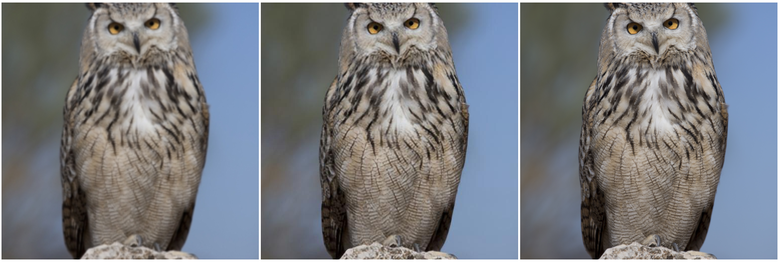
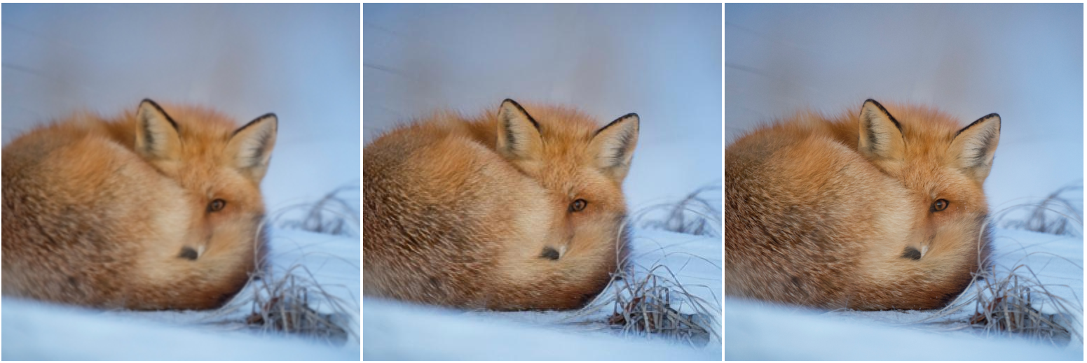
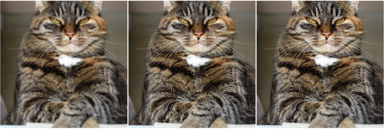
There are five examples below where I believe the model’s prediction (centre) is as good or very close to the target (right), the original ground truth image from the validation set. The model works well on animal features such as fur and eyes, with an eye being a very difficult task to sharpen and enhance.
Super resolution concluding example 1Super resolution concluding example 2Super resolution concluding example 3Super resolution concluding example 4Super resolution concluding example 5
There is one last example from the validation set where, in my opinion the model’s prediction (centre) is as better than the target (right), the original ground truth image from the validation set.
Super resolution concluding example 6, model prediction possibly better than the ground truth target?
Next steps
I’m keen to apply these techniques to different subject matters of images and to different sectors. If you think these super resolution techniques could help your industry or project then please get in touch.
I plan to move the model into a production web application, then possibly into a mobile web application.
I am in the process of training on larger sub-sets of the Image Net dataset, which contains many categories to produce an effective universal super resolution model, that performs well on any category of images. I am also in the process of training a greyscale version of the same datasets I trained on here, where the model is colourising the images.
I plan to try model architectures such as ResNet-50 and also a ResNet backbone with an Inception stem.
Ethical concerns
By hallucinating details that aren’t there in used in categories such as security footage, aerial photography or similar then generating an image from a low resolution image might take it further from the original real subject matter.
Imagine if facial features were changed subtlety but enough to identify a person by facial recognition who wasn’t actually there or a aerial photo is changed just enough that a building is recognised by another algorithm as being something other than it is. Diverse training data should help avoid this, although as super resolution methods improve it is a concern as is the lack of diverse training data used historically in the machine learning research community.
Fastai
Thank you to the Fastai team, without your courses and your software library I doubt I would have been able to carry out these experiments and learn about these techniques.


