Capacitance calculations in the COMSOL Multiphysics® software seem easy. If you only have two conductors, the recipe is simple: Take one conductor and set it to grounded, set the other as a terminal, and compute the solution. Then, a built-in variable delivers the capacitance. But what if you have more than two conductors, like in touchscreens, transmission lines, and capacitive sensors? If standard textbook terminology has you lost, follow along with this working example of calculating a capacitance matrix.
What Is Self-Capacitance?
Capacitance is the ability of a system to store electric charge. It can be defined by the amount of charge that a body needs in order to raise its electric potential by 1 volt against a grounded reference potential. In a linear system, this is
where Q is charge, V is potential difference relative to ground, and C is the capacitance.
Before we get to multiconductor systems, remember that by definition, even a single isolated conductor has a capacitance, defined relative to a grounded spherical shell at infinity. For the case of a conducting sphere, this self-capacitance is
We can use this formula to calculate, for example, the self-capacitance of planet Earth — it is roughly 710 microfarad.
Human bodies can also be charged up, as seen here.
Hence, the human body, too, exhibits self-capacitance (also called body capacitance). Depending on posture and the surrounding area, body capacitance is in the range of 100 picofarad and can even create a tingling sensation in humans. You can, for example, easily charge up your body capacitance to several thousand volts while brushing your hair in the morning. Make sure to be well grounded before starting the day!
Comparing Mutual and Maxwell Capacitance Matrices
In typical electrical systems, capacitances between several conductors are of most interest. Mutual capacitance, also referred to as parasitic or stray capacitance, is desired or undesired capacitance (a buildup of charge) that occurs between two charge-holding objects. If you bring a charged object near another object, the charge distribution on the first object will change due to the process of electrostatic induction (not to be confused with electromagnetic induction). Particularly in transmission systems, capacitive coupling between lines is often unintended and troublesome, as it can create noise.
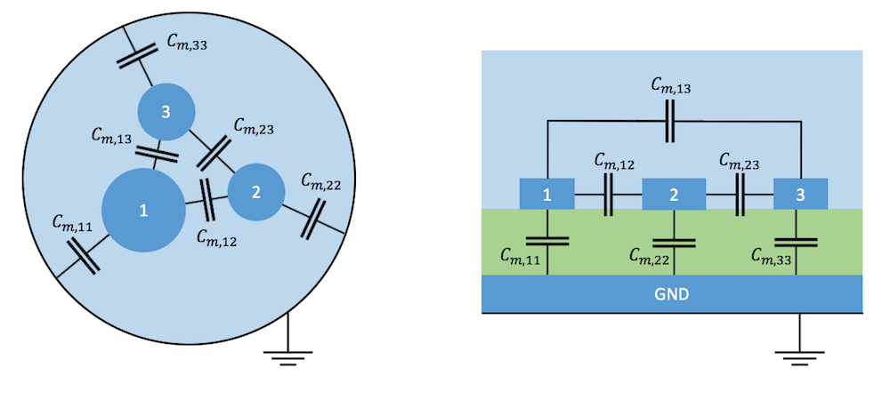
Typical examples of mutual capacitance in a shielded three-conductor cable (left) and between microstrip transmission lines over a ground plate (right). The transition from a continuous field model to a lumped model with discrete capacitors means to shrink the conductors to points while moving the charges at their surface to the plates of capacitors shown between them.
For convenience, it is possible to arrange mutual capacitances of a system of N conductors and one additional ground in matrix form:
The coefficients of this matrix, also called partial capacitances or lumped capacitances, are used in a circuit simulator when you reduce a physical system to a network of discrete elements.
In field theory, another matrix form is more common: the Maxwell capacitance matrix. Because the name is so similar and the coefficients are not identical, it is important to understand the relation between mutual and Maxwell capacitance matrices. The Maxwell capacitance matrix describes a relation between the charge of the ith conductor to the voltages of all conductors in the system.
The Maxwell capacitance matrix coefficient could be determined by measuring the charge on conductor 1, when only the potential and all other electrodes are grounded. Therefore, the matrix is also often called the ground capacitance matrix. Its inverse, , is referred to as the elastance matrix.
We can also calculate the total charge on conductor 1 by summing up the contributions from the self- and mutual capacitances as follows.
For a system with N conductors, the relation between the mutual and Maxwell capacitance matrices is then
You can easily tell a Maxwell capacitance matrix by its negative nondiagonal elements.
Working Example: Mutual Capacitance of Two Spheres
Now that we have a clear definition of the terminology, let’s explore how easy it is to calculate capacitance matrices for arbitrary systems of conductors in COMSOL Multiphysics. To feel solid ground under our feet, we’ll start with a system with a known analytical solution. (Did I mention that I love analytical solutions? Actually, whenever I start a new simulation project, I try to find a simple system with an analytic solution to reproduce.)
In our case, we can use a system consisting of two conducting spheres of radii a and b, separated by a distance c and a ground reference at infinity.
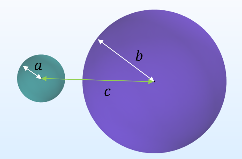
Closed-form expressions for such a system have been known since Maxwell’s times. I am referring to two readily available publications of de Queiroz (2003) and Lekner (2011). The expressions for the three Maxwell capacitance matrices are
where
You can easily declare these expressions as variables in COMSOL Multiphysics by using the sum operator:
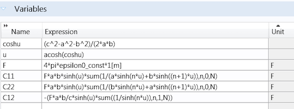
With a parametric sweep over N, we find that the series converges rapidly when the spheres are not too close to each other. We can safely set N to 10 for a given set of parameters: a = 0.1, b = 0.3, and c = 0.5.
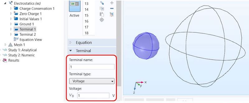
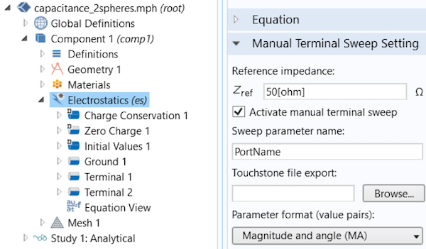
In order to calculate the capacitance matrix in the Electrostatics interface, we set a terminal condition to one sphere with a potential of 1 V.
Next, we duplicate the feature, apply it to the second sphere, and set the terminal name to 2. In order to calculate capacitance matrices, we need to apply different voltage or charge patterns to the terminals. For didactic reasons, we’ll discuss the traditional manual terminal sweep before introducing new, significantly faster technology that was released in version 5.3 of the COMSOL® software. While the new technology is faster in a large class of very common problems, the manual method is more general.
A manual terminal sweep is activated directly in the Electrostatics interface.
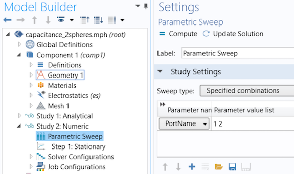
After declaring the Sweep parameter name in the Global Parameters section (PortName by default), you can then run a parametric sweep over PortName.
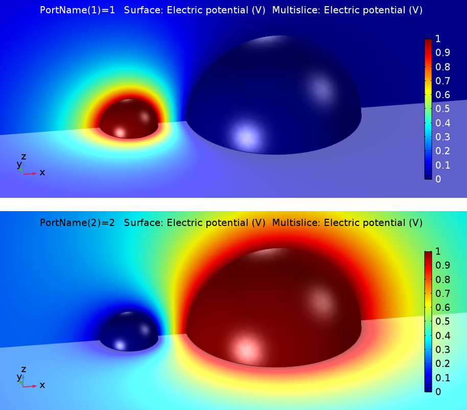
In the model, the COMSOL Multiphysics software sets one terminal to 1 V and all others to ground during the sweep, resulting in the following two solutions:
You can use Results > Global Matrix Evaluation to extract the capacitance matrices in different notations, including the Maxwell capacitance matrix and the mutual capacitance matrix.
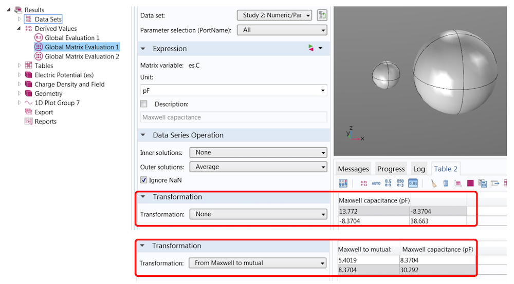
In this simple example, their relation is
If you are setting charge terminals instead of voltage terminals, the primary solution is the inverse capacitance matrix. A set of transformations are available that can help you convert the charge into the above-mentioned matrices.
Gain Speed with Stationary Source Sweeps and the Boundary Element Method
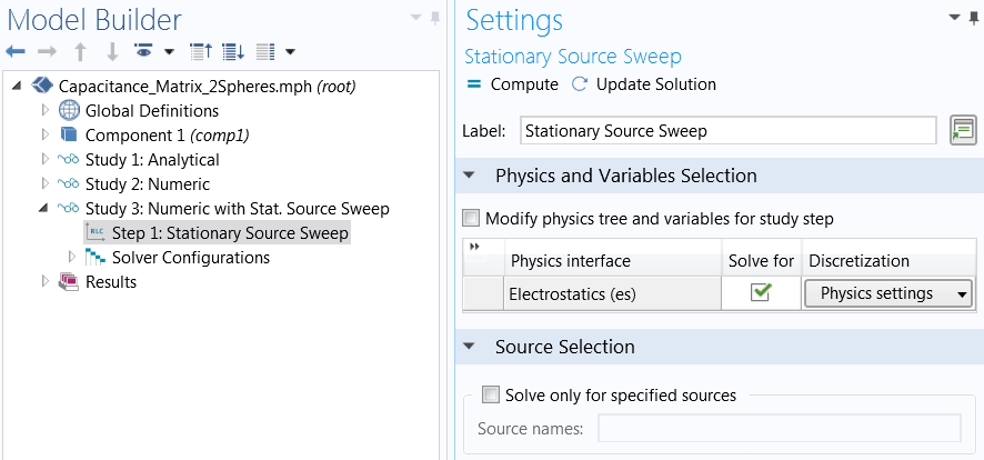
In COMSOL Multiphysics version 5.3, we have introduced many powerful new modeling methods. One feature particularly relevant to capacitance matrix calculations is the new Stationary Source Sweep study step.
In contrast to manual terminal sweeps, which use a parametric sweep for PortName, this new technology accounts for the fact that applying different charges or voltage patterns to the electrostatic system doesn’t change the system matrix of the underlying FEM equations, only their loads. This means that the matrix needs to be inverted only once and can be reused for all other load cases. This approach can dramatically reduce computational time, especially when the number of terminals is large or other parametric sweeps (e.g., for the geometry) are needed.
Even for a moderate number of terminals, like in the Touchscreen Simulator simulation app, the speed gain is surprising: I could reach a factor of 7.8 on my machine for this model with the same number of DOF!
The new Capacitive Position Sensor tutorial model uses the Stationary Source Sweep study step.
A stationary source sweep is also easier to set up. There is no need to activate a manual terminal sweep and define a PortName variable and a parametric sweep. All you need to do is select a study step. By default, the study will run through all terminals. Alternatively, you can define specified sources that you want to cover.
If the stationary source sweep is so powerful, then why do we keep the traditional approach at all?
There are cases where we appreciate a recalculation of the system matrix; for instance, in nonlinear or multiphysics problems or if meshes should be adapted for each terminal configuration. In such cases, a manual terminal sweep is a better method.
Another powerful feature that comes with version 5.3 of the COMSOL® software is the boundary element method (BEM) in electrostatics. Compared to FEM, where a mesh in all domains (including the surrounding air domain) is needed, BEM avoids meshing in the infinite void, which reduces the number of DOFs. You can learn more about combining BEM in electrostatics and capacitance matrix calculation in the Modeling a Capacitive Position Sensor Using BEM tutorial.
Can’t wait to learn more about the new BEM implementation? Read about how this method has already helped to simplify corrosion modeling in a previous blog post.
Concluding Thoughts on Capacitance Matrix Calculation
In this blog post, we have looked into the calculation of capacitance matrices, discussed the different terminologies, and provided a numerical solution for a well-known problem that has a closed-form solution. While the simple model presented here can provide a reference for your own models, the new features released in version 5.3 can help you to create large models with many terminals and additional parametric sweeps more efficiently.CONTACT COMSOL FOR A SOFTWARE EVALUATION
Additional Resources
- Browse these blog posts on capacitance and BEM:
References
- de Queiroz, A.C.M., 2003, “Capacitance Calculations“.
- Lekner, J., 2011, “Capacitance coefficients of two spheres”, Journal of Electrostatics 69(1):11-14.